Dynamic sheet tab names in formulas mean referring to sheet names dynamically in formulas. If you delve deeper, it involves switching tab names in formulas automatically or semi-automatically. By semi-automatically, I mean with the help of a drop-down menu or a helper cell.

To achieve dynamic sheet tab names in formulas, we must use the INDIRECT function. However, how you use the INDIRECT function is crucial.

The typical method is to enter all the sheet names in a drop-down menu and refer to this using INDIRECT. This is known as the helper cell approach.

But there is another approach, limited to sheet tab names such as dates, months, weekdays, etc. Yes! You can dynamically refer to sheet tab names in formulas without referring to any helper cell.

Use today’s or tomorrow’s dates as sheet names and get them automatically updated in formulas. By doing so, your formula will automatically refer to the newly added sheets based on the current date.

Dynamic Sheet Tab Names with Helper Cells (Semi-Dynamic)

In semi-dynamic sheet references, we will create a drop-down menu containing all your sheet tab names in a file.

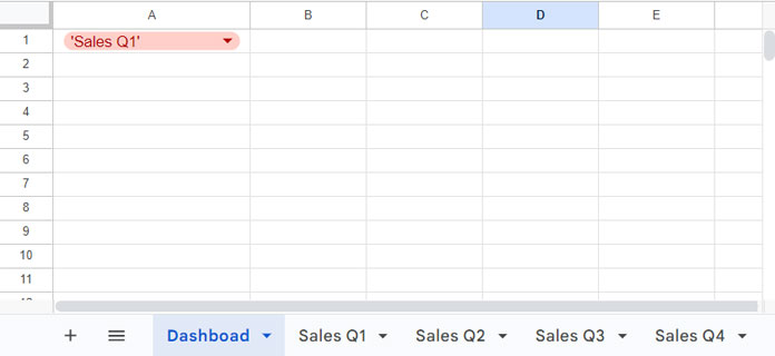
Assume you have four sheets in your file named “Sales Q1,” “Sales Q2,” “Sales Q3,” and “Sales Q4.”

You can refer to these sheets dynamically in formulas by selecting sheet names from a drop-down.

You can create the drop-down in any cell in that file, but for our testing, we will add a new sheet tab.

Adding a New Sheet Tab:

1. Click the + Add Sheet button at the bottom left corner of the Sheets window to add a new sheet.

Naming the New Tab:

1. Double-click the sheet name and name it. Here, I name it “Dashboard.”

Creating a Drop-down with Sheet Names:

1. Navigate to cell A1 in the Dashboard sheet.
2. Click Insert > Drop-down.
3. Replace the placeholder texts “Option 1” with ''Sales Q1' and “Option 2” with ''Sales Q2'. Click Add Another Item and enter ''Sales Q3'. If you have more sheets, add their names by clicking the Add Another Item button.

In step 3, when you enter sheet names, you should prefix each with two apostrophes and suffix with one apostrophe.

Using INDIRECT to View Content from Each Sheet:

Now, to view the content from each sheet, you can use INDIRECT as follows:

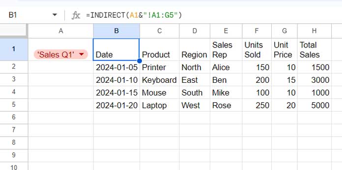
Instead of directly referring to A1:G5, combine the drop-down value in cell A1 with an exclamation mark, followed by the cell or range reference. Then wrap them with the INDIRECT function.

=INDIRECT(A1&"!A1:G5")

When you select another sheet name from the drop-down, it will return the data from the selected sheet.

Examples of Semi-Dynamic References:

Here are some formula examples:

SUM:

=SUM(INDIRECT(A1&"!G2:G5")) // sums the values in G2:G5 in the sheet selected in the drop-down

COUNTIF:

=COUNTIF(INDIRECT(A1&"!B2:B"),"Printer") // counts the occurrences of the text "Printer" in the range B2:B in the sheet selected in the drop-down

SUMIF:

=SUMIF(INDIRECT(A1&"!B2:B"), "Printer", INDIRECT(A1&"!G2:G")) // sums column G if column B matches "Printer" in the sheet selected in the drop-down

Referencing Sheet Tabs Dynamically Without Helper Cells

In the earlier example, I used a drop-down menu in cell A1, which means a helper cell was used to get the dynamic sheet tab names to work in formulas.

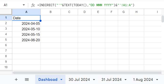
Here is a different approach. If your sheet tab names are dates, you can use this fully dynamic method to refer to them using the TODAY date function within INDIRECT.

When naming the tabs, use a consistent date format. I suggest using “DD MMM YYYY,” for example, “31 Jul 2024.”

Examples of Fully Dynamic References:

To dynamically refer to today’s sheet, use the following formula:

=INDIRECT("'"&TEXT(TODAY(),"DD MMM YYYY")&"'!E2:E")

For example:

=COUNTIF(INDIRECT("'"&TEXT(TODAY(),"DD MMM YYYY")&"'!E2:E"), ">100")

Note: Replace E2:E with the range or cell reference you want.

The formulas in the ‘Dashboard’ will automatically refer to the sheet tab name corresponding to today’s date.

You can use TODAY()-1 to refer to yesterday’s date sheet if needed.

What About Using Month Names as Tab Names and Dynamically Referring to the Current Month?

To dynamically refer to the current month’s sheet, use the following formula:

=INDIRECT("'"&TEXT(TODAY(),"MMMM")&"'!A1:A")

Remember to use full month names as the tab names in your sheets.

These are additional examples of using dynamic sheet tab names in Google Sheets formulas.

Dynamic Sheet Tab Name References and Their Common Errors

You may encounter issues when using dynamic sheet tab names associated with non-existing sheet names.

In semi-dynamic references, errors may arise due to typos in the sheet names specified in the drop-down menu or if a sheet is accidentally deleted.

In fully dynamic references using dates, errors typically occur when referring to non-existent sheet names.

The errors may vary depending on the formula. Here are the two most common errors associated with dynamic sheet tab names in formulas:

• #REF – Invalid cell or range reference
• #N/A – Argument must be a range

For semi-dynamic references, check for typos in the original sheet tab names and those used in the drop-down menu.

For fully dynamic references, verify that the date formatting used in the formula matches the date format in the sheet tab names.

If they match and the formula still returns an error, try re-entering the formula to refresh it.

Resources

• Dynamic Sheet Names in IMPORTRANGE in Google Sheets
• Combine Data Dynamically in Multiple Tabs Vertically in Google Sheets
• Dynamically Combine Multiple Sheets Horizontally in Google Sheets
• How to Hide Tabs from Specific People in Google Sheets
• Print Continuous Page Numbers Across Sheet Tabs in Google Sheets
• How to Include Future Sheets in Formulas in Google Sheets