Recently, one of my readers asked about the possibility of using dynamic ranges in the GROWTH function in Google Sheets. With the help of the FILTER function, you can apply dynamic ranges not only in the GROWTH function but also in the TREND and FORECAST functions.
Don’t be puzzled by the function names. My Google Sheets functions guide provides detailed explanations of these functions and their applications. Here’s a quick overview of their purposes:
- FORECAST: Used to predict future values based on historical data. It’s commonly applied to estimate a future value using past data points.
- TREND: Fits a linear trend line to your data and extends it beyond the existing values. This function helps forecast a range of future values based on a linear pattern.
- GROWTH: Projects future values by fitting an exponential curve to your existing data. Ideal for data that shows exponential growth or decay.
This post explores how to use dynamic ranges for known_data_x, known_data_y, and new_data_x in exponential growth (GROWTH), linear trend (TREND), and linear regression (FORECAST) calculations in Google Sheets.
Typically, you cannot use infinite ranges like A2:A or B2:B directly in these functions. However, you can leverage the FILTER function to work with dynamic data ranges in GROWTH, TREND, and FORECAST functions.
Understanding the Concept
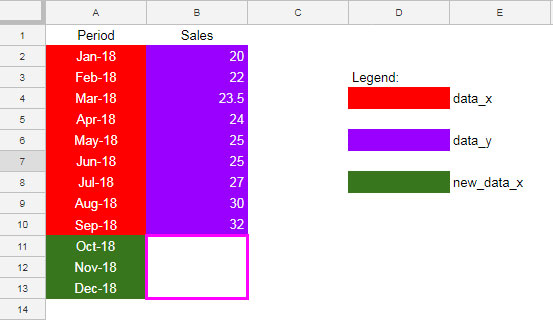
In the screenshot below, I’ve highlighted data_x, data_y, and new_data_x.

Refer to the legends and dataset for color coding, which helps identify data_x, data_y, and new_data_x in the GROWTH, TREND, and FORECAST functions.
The ranges for data_x and data_y contain existing values. Sometimes, these might be referred to as known_data_x and known_data_y. We need to find values corresponding to new_data_x.
First, let’s understand the fixed data ranges used in the three functions:
Exponential Growth:
Syntax of the GROWTH Function: GROWTH(known_data_y, [known_data_x], [new_data_x], [b])
Formula:
=GROWTH(B2:B10, A2:A10, A11:A13)Linear Trend:
Syntax of the TREND Function: TREND(known_data_y, [known_data_x], [new_data_x], [b])
Formula:
=TREND(B2:B10, A2:A10, A11:A13)Linear Regression:
Syntax of the FORECAST Function: ArrayFormula(FORECAST(x, data_y, data_x))
Formula:
=ArrayFormula(FORECAST(A11:A13, B2:B10, A2:A10))In these examples, I’ve used fixed (closed) data ranges. Now, let’s explore how to use dynamic data ranges in the GROWTH, TREND, and FORECAST functions in Google Sheets.
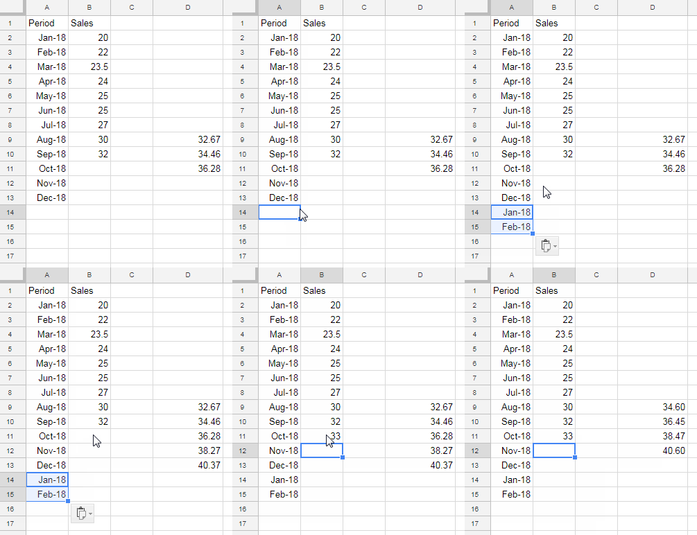
Suppose the data ranges are updated either by other formulas or manually by users. In such cases, the ranges may change frequently, causing issues with fixed ranges as they might not include new values.
For instance, with the initial formulas, the data ranges are:
data_x: A2:A10data_y: B2:B10new_data_x: A11:A13
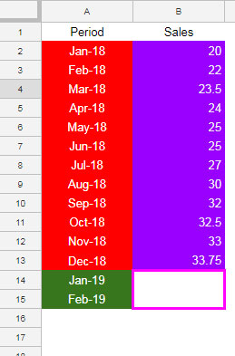
If new values are added, the updated ranges might be:
data_x: A2:A13data_y: B2:B13new_data_x: A14:A15

Can we accommodate these changes without altering the formula?
Yes! Let me explain how to use dynamic data ranges in the GROWTH, TREND, and FORECAST functions in Google Sheets, starting with the GROWTH function.
Using Dynamic Ranges with the GROWTH Function in Google Sheets
As mentioned, using an expanding range in the GROWTH function allows you to handle dynamic or infinite data for data_x, data_y, and new_data_x. For example:
Standard GROWTH Formula:
=GROWTH(
   B2:B10,
   A2:A10,
   A11:A13
)
Dynamic Range Formula:
=GROWTH(
   FILTER(B2:B, B2:B<>""),
   FILTER(A2:A, B2:B<>""),
   FILTER(A2:A, (N(B2:B)=0)*(A2:A>0))
)
In the dynamic range formula, FILTER functions adjust the ranges to include all relevant data points, enabling the GROWTH function to predict values based on the most current data.

Formula Explanation
Let me break down the formula according to the GROWTH function’s syntax:
GROWTH(
   known_data_y,
   known_data_x,
   new_data_x
)
Generic Formula Using FILTER within GROWTH:
=GROWTH(
   FILTER(known_data_y, known_data_y<>""),
   FILTER(known_data_x, known_data_y<>""),
   FILTER(known_data_x, (N(known_data_y)=0) * (known_data_x>0))
)
Here’s what each part means:
known_data_y: Filters the range B2:B to exclude blanks (B2:B<>"").known_data_x: Filters the range A2:A, ensuring corresponding B2:B values are not blank (B2:B<>"").new_data_x: Filters A2:A where B2:B is equal to zero and A2:A is greater than 0 (N(B2:B)=0andA2:A>0).
This logic helps dynamically adjust the data ranges.
Regarding the new_data_x filter, you might wonder about the logic used. The formula employs OR logic in the FILTER function, which is explained in more detail in my tutorial: How to Use AND, OR with Google Sheets Filter Function.
Using this method, you can apply dynamic or infinite data ranges in the GROWTH function within Google Sheets.
Dynamic Range in the TREND Function
For the TREND function, you can follow a similar approach as with the GROWTH function. Here’s how to apply a dynamic range in the TREND function in Google Sheets.
Formula:
=TREND(
   FILTER(B2:B, B2:B<>""),
   FILTER(A2:A, B2:B<>""),
   FILTER(A2:A, (N(B2:B)=0) * (A2:A>0))
)
Syntax:
TREND(
   known_data_y,
   known_data_x,
   new_data_x
)
In this formula, only the function name changes. For a better understanding of how this works, refer to the dynamic range example for the GROWTH function.
Dynamic Range in the FORECAST Function
The approach for creating a dynamic range in the FORECAST function is similar to TREND and GROWTH, with a few differences.
In this case, the arguments are positioned differently, and since the FORECAST function isn’t an array formula by default, I’ve used the ArrayFormula function.
Formula:
=ArrayFormula(FORECAST(
   FILTER(A2:A, (N(B2:B)=0) * (A2:A>0)),
   FILTER(B2:B, B2:B<>""),
   FILTER(A2:A, B2:B<>"")
))
Syntax:
ArrayFormula(FORECAST(
   x,
   data_y,
   data_x
))
Conclusion
If your data range—both known_data_x and known_data_y—continues to grow, and there are updates to new_data_x (which is likely), you can apply the approach outlined above.
The key to using dynamic data ranges in the GROWTH, TREND, and FORECAST functions in Google Sheets lies in how you utilize the FILTER function.
Once you understand FILTER, you’ll easily master how to use dynamic or infinite ranges in these functions. Thanks for reading, and happy learning!


