This post explains the use of the DSTDEVP function (database) in Google Sheets. In this, “D” stands for database, “STDEV” for standard deviation, and “P” for the population.

When we consider standard deviation calculations in Google Sheets, we can see functions under two categories – Database and Statistical.

The former category function supports applying the calculation on selected entries in the dataset, whereas the latter doesn’t.

So in the statistical functions, we may be required to use QUERY or FILTER to apply criteria. So, here, the database functions scores.

As mentioned above, the DSTDEVP function in Google Sheets is coming under the database category.

The problem with these types of functions is we can use them only in a well-formatted dataset.

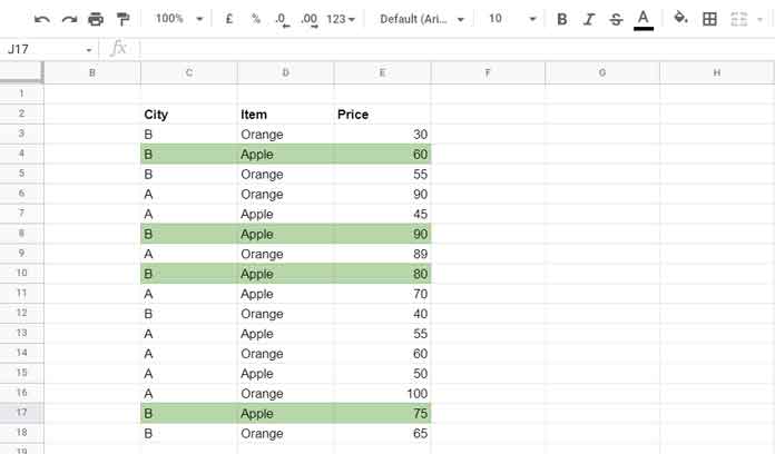
A well-formatted dataset is a multi-column array/range containing field labels/column names in the topmost row. We can consider the below table as an example.

As a side note, in a blank cell, start typing =st to see the statistical and =dst for all the database functions. Most of them are already featured on this page – Google Sheets function Guide.

Introduction

Before going to the function syntax and formula examples, let’s get a basic idea of the calculation.

Please see the highlighted records in the table above.

Let’s see how to calculate the standard deviation of the values in the “Price” column of those rows without using the DSTDEVP function in Google Sheets.

1. Find the mean as below.

=(60+90+80+75)/4

Result: 76.25

2. For each data point, subtract the mean, square the result and sum it.

=(60-76.25)^2+(90-76.25)^2+(80-76.25)^2+(75-76.25)^2

Result: 468.75

3. Divide by the number of data points.

=((60-76.25)^2+(90-76.25)^2+(80-76.25)^2+(75-76.25)^2)/4

Result: 117.1875

4. Take the square root and the result will be 10.82.

Syntex of the DSTDEVP Function in Google Sheets

Syntax:

DSTDEVP(database, field, criteria)

Arguments:

database: The structured data/the well-formatted dataset, as explained at the beginning of this tutorial.

field: The column index number contains the value to calculate. We can either use the corresponding field label entered within double quotation marks or the column index number itself (relative position of the calculation column in the database).

criteria: To specify which records to include in the calculation. It must be entered as an array, and that must at least contain one field label and one cell below it.

Formula Examples

Similar to all the other database functions in Google Sheets, we have the comfort of providing the criteria as an array reference or hardcode within the formula.

Here are a few formulas. The first formula takes one criterion, whereas the second one takes two criteria.

For the example purpose, let’s use the above same structured table.

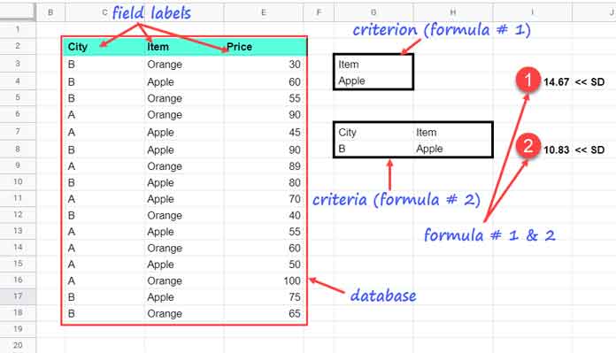
Point # 1 Formula (One Criterion):

=dstdevp(C2:E18,"Price",G3:G4)

Point # 2 Formula (Two Criteria):

=dstdevp(C2:E18,"Price",G7:H8)

Criteria Hardcoded in DSTDEVP Function in Google Sheets

Google Sheets all database functions are very flexible when it comes to using conditions. In the above two DSTDEVP function examples, I have specified the criteria as an outside array.

See how can we use that within the formula.

Point # 1 Formula:

=dstdevp(C2:E18,"Price",{"Item";"Apple"})

Point # 2 Formula:

=dstdevp(C2:E18,"Price",{"City","Item";"B","Apple"})

If you are not well conversed in creating an array as above using the Curly Brackets, please read this guide – The Ultimate Guide to Using Criteria in Database Functions in Google Sheets.

That’s all about how to use the DSTDEVP function in Google Sheets. I hope you have enjoyed your stay!