When working with date-based data in Google Sheets, you often need summaries at multiple levels—yearly, quarterly, and monthly—without creating extra helper columns in your source data.
For example, imagine a credit card or bank statement covering multiple financial years. You want to:
- View totals by Year
- Drill down to Quarter
- Further drill down to Month
All of this can be done using a single date column in a Pivot Table.
Google Sheets Pivot Tables support date grouping, which automatically creates a date hierarchy—no need to add Year, Quarter, or Month columns to your dataset.
This tutorial shows exactly how to drill down and drill up a date column in a Pivot Table using built-in date grouping.
This article is part of the larger guide: Pivot Table Formatting, Output & Special Behavior in Google Sheets (hub)
Step 1: Create the Pivot Table
- Select your source data (for example,
A3:F13) - Go to Insert → Pivot table
- Choose New sheet and click Create
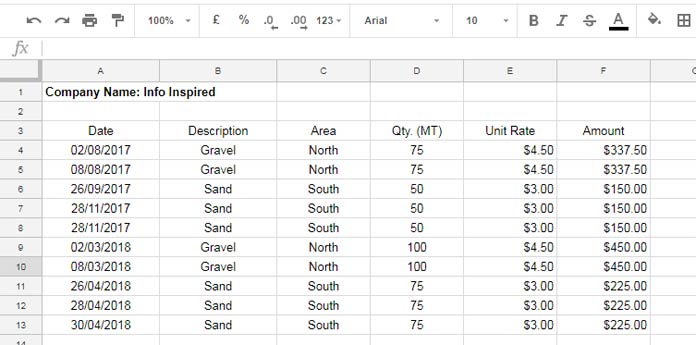
In the Pivot table editor:
- Rows → Date
- Values → Qty. (or Amount)
- Columns → Description (optional)
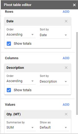
At this stage, dates appear at their lowest level, so there’s nothing to drill down yet.
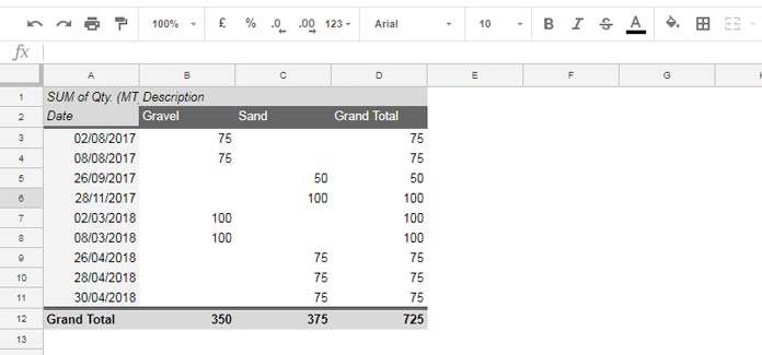
Step 2: Define the Date Hierarchy (Grouping)
To enable drill-down, the date column must be grouped.
Decide the hierarchy first. Common options include:
- Year → Quarter → Month (used here)
- Year → Month
- Quarter → Month
- Month → Day of week
In this example, we’ll use a three-level hierarchy: Year → Quarter → Month
Step 3: Drill Down the Date Column in the Pivot Table
Group Dates by Year
- Right-click any date in the Pivot Table
- Select Create pivot date group → Year
A new Year level appears in the Rows area.
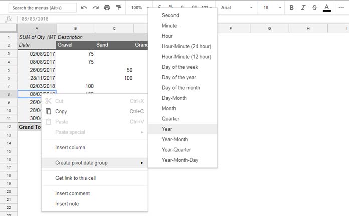
Add the Quarter Level
- Open the Pivot table editor
- Under Rows, click Add → Date
- Right-click a date in the new column
- Select Create pivot date group → Quarter
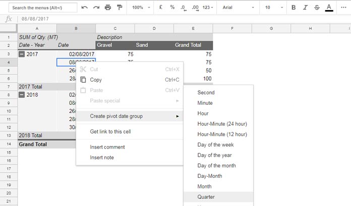
Add the Month Level
Repeat the same process:
- Add Date again under Rows
- Right-click a date
- Select Create pivot date group → Month
Your Pivot Table now shows a collapsible date hierarchy.
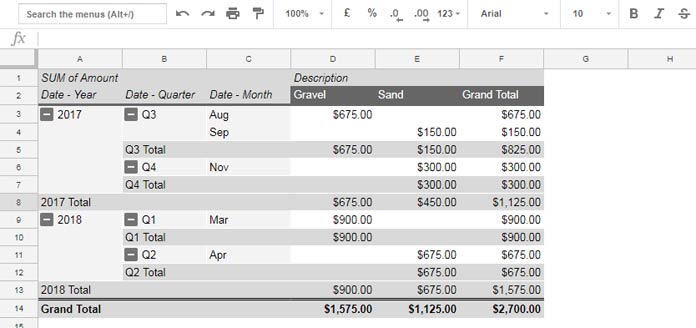
How to Drill Down or Drill Up Dates
- Click ➖ (minus) to collapse a level
- Click ➕ (plus) to expand it
You can move seamlessly between Year, Quarter, and Month views.
You may also add Day of week as an additional level, but it’s optional and depends on reporting needs.
Why This Method Is Better Than Helper Columns
- No extra Year / Month / Quarter columns needed
- Cleaner source data
- Fully dynamic reporting
- Works with any valid date column
Related Guide: Pivot Table Formatting, Output & Special Behavior
If you’re working extensively with Pivot Tables, this tutorial is part of a broader resource covering:
- Formatting behavior
- Output quirks
- Special Pivot Table limitations
👉 Pivot Table Formatting, Output & Special Behavior in Google Sheets


I follow your posts on google sheets regularly and also a subscriber of your blog. I have an interesting problem/challenge for you that could be a topic for your post also.
Kindly go through a post http://www.contextures.com/xlPivot-Filter-Source-Data.html. It provides a code for excel pivot table by which double-clicking opens the data source with filters showing just the rows that make the value for the double-clicked cell.
I find this feature very very useful and has been looking for a script for Google Sheets. But did not have any luck so far.
There is a data drill feature in Google Sheets pivot that throws such rows but only on a new Sheet, not the filtered data source that I am looking for.
I feel there should be some way to replicate the code in the above post for google sheet also or maybe some round-about way.
After a lot of searching, I feel you are the only person who can probably help. Request you to kindly write a post on this problem and provide some solution.
Hi, S K Srivastava,
When you double click on any aggregated values in Sheets Pivot Table, Google Sheets open a new tab to show the details associated with it. I understand you do not like this feature and want the details within the Pivot Table Sheet tab.
For this, I can only think about a formula based workaround as I’m not familiar with Apps Script. One thing I can recommend you is using a Query.
=query(A3:B,"Select * where A='"&E3&"'")Change E3 in the formula.
If you may not like such a solution you might find lucky asking your question on the Google Community Forum.
https://support.google.com/docs/threads?hl=en&thread_filter=(category:docs_sheets)
Please post your question there. There are lots of contributors who can help you with this.
You can also find me there 😀
Best,
Prashanth KV