


")


")

")
")
 in Excel & Google Sheets")


The DOLLARFR function in Google Sheets converts a decimal dollar value (like 10.25) into a fractional-style format, based on a specified denominator. For example, DOLLARFR(10.25, 8) returns 10.2, where the “.2” represents 2/8 of a dollar, not two-tenths. This is especially useful in finance, where prices—like bond quotes—are often written in fractions instead of decimals.
This function performs the opposite of what the DOLLARDE function does.
Note: Avoid using the result of the DOLLARFR formula in further calculations, as it returns a decimal-looking value that actually represents a fractional price. If you need to use the result for further math or charts, convert it back to decimal using DOLLARDE.
Let’s go over the syntax and examples to help you understand how to use this financial function in Google Sheets.
Syntax of DOLLARFR in Google Sheets
DOLLARFR(decimal_price, unit)Arguments:
- decimal_price – The price in decimal form (e.g., 10.25).
- unit – The denominator for the fraction (e.g., 4 for quarters, 8 for eighths, 16 for sixteenths, 32 for thirty-seconds).
Both arguments are required for the function to work properly.
DOLLARFR vs DOLLARDE (Example Included)
As mentioned above, the DOLLARFR function works the opposite way of DOLLARDE.
Let’s start with this example:
- Fractional Price: 10.20
- Unit: 8
=DOLLARDE(10.2, 8)Result: 10.25
Calculation: 10 + 2/8 = 10.25
Now reverse it using DOLLARFR:
- Decimal Price: 10.25
- Unit: 8
=DOLLARFR(10.25, 8)Result: 10.20
Explanation: Converts 10.25 into a value read as 10 and 2/8.
Real-Life Use Case: When to Use DOLLARFR
The DOLLARFR function is particularly useful in finance, especially in the bond market, where prices are traditionally quoted in fractions of a dollar.
For example, a bond might be quoted as $101-04, which means $101 and 4/32. In decimal form, this would be $101.125.
To convert it to the fractional style commonly seen in bond quotes:
=DOLLARFR(101.125, 32)Result: 101.04
This makes the price more readable for clients or reporting, aligning with industry standards.
Pro Tip: Use DOLLARFR for display/reporting purposes only. If you need to calculate gains or returns, convert it back to decimal with DOLLARDE.
Use cases include:
- Financial analysts preparing reports
- Accountants reviewing investment statements
- Brokers quoting traditional prices
Additional Examples of the DOLLARFR Function
Here’s a table with more examples to help you understand different unit scenarios:
| Decimal Price | Unit | Result | Formula | Description |
|---|---|---|---|---|
| 10.25 | 8 | 10.20 | =DOLLARFR(10.25,8) | Converts 10.25 to 10 and 2/8 |
| 11.25 | 16 | 11.04 | =DOLLARFR(11.25,16) | Converts 11.25 to 11 and 4/16 |
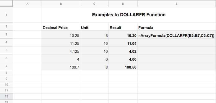
Convert Multiple Values with ARRAYFORMULA
To apply DOLLARFR to multiple rows at once, use it with ARRAYFORMULA.
Assuming column A has decimal prices and column B has unit values:
=ARRAYFORMULA(DOLLARFR(A2:A, B2:B))This will return a column of fractional prices.
DOLLARFR Function – Error Values
Here are common error scenarios you might encounter:
- #VALUE! – One or both arguments are non-numeric text.
- #DIV/0! – The unit is 0 or between 0 and 0.99.
- #NUM! – The unit is a negative number.
- Decimal Unit – Non-integer units (like 1.5) are truncated to integers (1.5 becomes 1).
- Text-formatted numbers – These will be auto-converted and still work in the formula.
Conclusion
The DOLLARFR function in Google Sheets is a helpful tool for converting decimal dollar prices into fractional notation—especially when dealing with financial data like bond pricing. While it’s not suitable for calculations, it plays an important role in formatting and reporting.
If you frequently work with bond quotes or fractional pricing, mastering this function is a small but valuable step.