This article is a child post of the hub Date Logic in QUERY Function in Google Sheets. It explains how to work with date values (date serial numbers) in Google Sheets QUERY—a topic that often causes confusion, especially when working with imported data or DateTime formulas.

What Are Date Values (Date Serial Numbers)?

In Google Sheets, every date is stored internally as a number, known as a date serial number. This number represents the count of days since December 30, 1899.

Example

The date 01/11/2020 (1st November 2020) has the date value 44136 in Google Sheets.

You can verify this in either of the following ways:

• Enter the date in any cell, then go to Format > Number > Number.
• Use the formula: =DATEVALUE("01/11/2020")
  The date format (dd/mm/yyyy or mm/dd/yyyy) depends on your spreadsheet locale.

Why Do We Sometimes Get Date Values Instead of Dates?

You may encounter date serial numbers instead of formatted dates due to:

• Imported data (CSV files, API results, or external connections)
• Formula output, such as INT(), arithmetic operations on dates, or array expressions

Since date values behave differently from formatted dates inside QUERY, it’s important to know how to handle them correctly.

This tutorial is part of the Date Logic in QUERY hub, which covers date criteria, month-based filtering, and DateTime handling in Google Sheets QUERY.

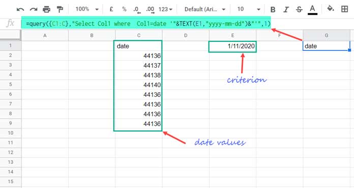
Basic QUERY with a Date Column

To filter a date column using QUERY, you normally use a date literal.

=QUERY({C1:C},"select Col1 where Col1 = date '"&TEXT(E1,"yyyy-mm-dd")&"'",1)

This formula filters dates in C1:C that match the date in E1 (for example, 01/11/2020).

What Happens If Dates Are Converted to Date Values?

Now, manually convert the dates in C2:C to numbers:

• Select C2:C
• Go to Format > Number > Number

You’ll notice that the QUERY formula now returns only the header, with no matching values.

Why?
Because QUERY treats numeric date values differently from date literals.

Handling Date Values When Imported Data Contains Date Values

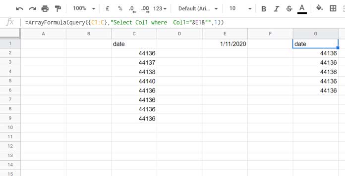
If your imported data already contains date serial numbers, you have two valid approaches.

Option 1: Use a Number Literal Instead of a Date Literal

Assume:

• C2:C contains date serial numbers (numeric values)
• E1 contains a date (formatted as a date, not manually converted to a number)

In this case, you must use a number literal in the QUERY condition instead of a date literal.

=ARRAYFORMULA(QUERY({C1:C},"select Col1 where Col1 = "&E1&"",1))

Here:

• E1 contains a date, but Google Sheets automatically treats it as its underlying date serial number when concatenated into the QUERY string.
• We therefore use a number literal (for example, Col1 = 44138) rather than a date literal.

This replaces the usual date-literal syntax:

Col1 = date '"&TEXT(E1,"yyyy-mm-dd")&"'

which does not work when the data column contains date serial numbers instead of formatted dates.

Related: Examples of the Use of Literals in QUERY in Google Sheets

Option 2: Reformat Date Values Using the Format Menu

If the date values exist in a physical column, you can simply:

• Select the column
• Go to Format > Number > Date

Once converted back to dates, the standard QUERY with a date literal will work:

=QUERY({C1:C},"select Col1 where Col1 = date '"&TEXT(E1,"yyyy-mm-dd")&"'",1)

When Date Values Are Generated by a Formula (Expressions in QUERY)

In some cases, date values are produced by a formula rather than stored in a column.

Example

=ARRAYFORMULA(INT(C2:C))

Since this is an expression, you cannot use the Format menu to convert the values back to dates.

Use Numeric Literals in QUERY

=ARRAYFORMULA(QUERY(HSTACK(INT(C2:C),D2:D), "select Col1, Col2 where Col1 = "&E1&"",0))

This formula filters column C where the value matches E1, and the output includes the matching rows from columns C and D.

Key Takeaways

• Google Sheets stores dates as numeric serial values.
• QUERY requires number literals when working with date values.
• Formula-generated date values must be handled inside QUERY, not via formatting.

That’s all about using date values (date serial numbers) in Google Sheets QUERY.

Thanks for reading, and enjoy exploring date logic in QUERY!