By default, when you use the PIVOT clause in a Google Sheets QUERY, the pivoted column headers are sorted alphabetically (A–Z). But what if you want them in a custom order, like "Q2", "Q1", "Q3" or "High", "Medium", "Low"?

This tutorial shows you how to use the XMATCH function to sort QUERY pivot column headers in a custom order — including cases with more than one aggregation column.

Related Tutorials

We’ve previously covered related sorting use cases in Google Sheets:

• Custom Sort Order in Google Sheets QUERY – Focus: Sorting rows in a custom order.
• How to Sort Pivot Table Columns in the Custom Order in Google Sheets – Focus: Built-in Pivot Tables (from the Insert menu), not QUERY.
• Sort QUERY Pivot Headers in Descending Order in Google Sheets – Focus: Sorting pivot headers in descending order (e.g., Z–A, latest to earliest).

This guide is different — it shows how to override the default alphabetical A–Z sort and reorder QUERY pivot headers manually using a custom order.

Example 1: Custom Sort QUERY Pivot Headers with One Aggregation Column

Let’s start with a basic example using this sample data in A1:C10:

Assume you want a pivot table showing monthly sales per region.

Here’s the standard QUERY:

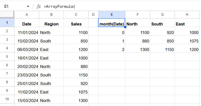
=QUERY(A1:C, "select month(A), sum(C) where A is not null group by month(A) pivot B", 1)

This will sort the pivot headers (regions) alphabetically:

Note: The month() function in Google Sheets returns months numbered from 0 (January) to 11 (December). To get standard month numbers from 1 to 12, use month(A) + 1 instead of month(A) in your QUERY formula.

But suppose you want to manually reorder the pivot columns as "North", "South", "East". Here’s how:

=ArrayFormula(
   LET(
      qry, QUERY(A1:C, "select month(A), sum(C) where A is not null group by month(A) pivot B", 1), 
      order, HSTACK("*Date*", "North", "South", "East"), 
      CHOOSECOLS(qry, XMATCH(order, chooserows(qry, 1), 2))
   )
)

How It Works

• qry: Stores the QUERY result.
• order: Specifies your custom order using HSTACK. Include the group column (with wildcard *Date*) followed by your desired header order.
• XMATCH: Finds the position of your desired column headers in the original result.
• CHOOSECOLS: Selects columns in your specified order.

This is how you reorder QUERY pivot column headers manually using XMATCH.

Example 2: Custom Sort QUERY Pivot Headers with Multiple Aggregation Columns

Now, let’s say you want to analyze both Quantity and Amount in your pivot.

Here’s the new sample data:

Here’s the regular pivot query:

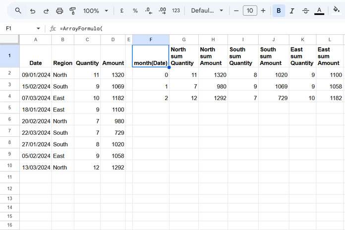
=QUERY(A1:D, "select month(A), sum(C), sum(D) where A is not null group by month(A) pivot B", 1)

This returns pivot headers in default alphabetical order:

Now let’s set a custom sort order for QUERY pivot headers:

=ArrayFormula(
   LET(
      qry, QUERY(A1:D, "select month(A), sum(C), sum(D) where A is not null group by month(A) pivot B", 1), 
      order, HSTACK("*Date*", "North*Quantity", "North*Amount", "South*Quantity", "South*Amount", "East*Quantity", "East*Amount"), 
      CHOOSECOLS(qry, XMATCH(order, chooserows(qry, 1), 2))
   )
)

Key Points:

• Use * as a wildcard for matching parts of the headers, e.g., "North*Quantity" matches "North sum Quantity".
• The order HSTACK should reflect the desired order of regions, each repeated for every aggregation column.

This method works even with multiple aggregation columns, allowing full control over QUERY pivot header ordering.

FAQs

❓ What about multiple group columns?

If you have more than one group column, specify both (or more) labels in the order array with wildcards around them like "*Product*", "*Date*".

❓ Can I rename the custom-sorted pivot headers?

Yes! Wrap the final formula in another QUERY to use the label clause, or use SUBSTITUTE to remove or rename parts like "sum".

❓ Can I custom sort QUERY pivot headers from IMPORTRANGE data?

Absolutely. Just refer to columns using Col1, Col2, etc., instead of A, B, C. Your QUERY will still work with XMATCH and CHOOSECOLS.

SAMPLE SHEET