There is no built-in function in Google Sheets to directly calculate the current or previous quarter from a given date or a list of dates. While you can use the QUARTER() scalar function in QUERY, it only works for calendar years (Jan–Dec) and doesn’t support fiscal years that start in other months.

With dynamic formulas, however, you can automatically calculate both the current quarter and the previous quarter based on TODAY(). The best part is that these formulas are flexible — you can define the starting month of your financial year, making them useful for both calendar years and custom fiscal years.

This approach is especially handy if you:

• Prepare recurring financial or sales reports
• Compare quarter-on-quarter performance
• Work with fiscal years that don’t follow Jan–Dec

By setting your own start month, the formulas adapt seamlessly to either standard calendar quarters (Jan–Mar, Apr–Jun, etc.) or fiscal quarters (e.g., Apr–Jun = Q1).

In this tutorial, you’ll learn how to:

• Get the current and previous quarter automatically using TODAY()
• Mark a list of dates with TRUE/FALSE flags for current or previous quarter
• Filter or summarize your data by quarter using QUERY for quick insights

Why Automating Quarters in Google Sheets Matters

Quarters are a natural way to break down performance in finance, sales, and project management, but updating them manually is error-prone and time-consuming.

By automating quarter calculations in Google Sheets, you can:

• Keep reports always current without manual edits
• Instantly filter or summarize data by quarter
• Support both calendar and fiscal year reporting

In short, automating quarters saves time, improves accuracy, and ensures your reports are always up to date.

Formula for Current Quarter in Google Sheets (Using TODAY())

Here’s the formula to return the current quarter in Google Sheets, based on today’s date:

=LET(
  dt, TODAY(), 
  start, 1, 
  fqtr, INT(MOD(MONTH(dt)-start, 12)/3+1), 
  fqtr
)

Enter this into any cell, and it will return the current quarter for the calendar year.

Adapting for Fiscal Years

To adjust this formula for fiscal years, change the start value to the month number when your financial year begins. For example:

• Use 1 → Jan–Dec calendar year
• Use 4 → Apr–Mar fiscal year (Apr–Jun = Q1, Jul–Sep = Q2, etc.)

👉 The logic stays the same; only the start month changes.

Formula for Previous Quarter in Google Sheets (Using TODAY())

Once you have the current quarter, finding the previous quarter is simple. Here’s the formula:

=LET(
  dt, TODAY(),
  start, 1, 
  fqtr, INT(MOD(MONTH(dt)-start, 12)/3+1),
  IF(fqtr=1, 4, fqtr-1)
)

This formula returns the previous quarter for the calendar year.

👉 To adapt for fiscal years, use the same adjustment as before: change start to your financial year’s first month (e.g., 4 for April).

Mark Dates as Current or Previous Quarter (TRUE/FALSE)

Finding the current or previous quarter is useful, but it becomes even more powerful when applied to a list of dates. By adding helper columns, you can mark whether each date falls in the current quarter or the previous quarter using TRUE/FALSE values.

This makes it easy to filter or summarize data without manual sorting.

Assume you have dates in column A2:A.
In B2, enter this formula to mark the current quarter:

=ArrayFormula(
  LET(
    dt, A2:A, 
    start, 1, 
    fqtr, INT(MOD(MONTH(dt)-start, 12)/3+1), 
    fyrs, YEAR(dt)-(MONTH(dt)<start), 
    fqtrT, INT(MOD(MONTH(TODAY())-start, 12)/3+1), 
    fyrst, YEAR(TODAY())-(MONTH(TODAY())<start), 
    DATE(fyrs, fqtr, 1)=DATE(fyrsT, fqtrT, 1)
  )
)

Formula Explanation

• start, fqtr, fyrs → calculate the quarter and year for each date in column A
• fqtrT, fyrsT → calculate the quarter and year for today’s date
• DATE(fyrs, fqtr, 1) → builds a reference date from quarter + year (e.g., all Q1 2025 dates become 01/01/2025)
• DATE(fyrsT, fqtrT, 1) → builds a reference date for the current quarter
• Comparison (=) → outputs TRUE if the date is in the current quarter, FALSE otherwise

Adapting for Previous Quarter

To mark the previous quarter, make one small change to the formula.
Replace:

DATE(fyrsT, fqtrT, 1)

with:

IF(fqtrT=1, DATE(fyrsT-1, 4, 1), EDATE(DATE(fyrsT, fqtrT, 1), -1))

This adjustment shifts the “quarter key date” for TODAY() back by one quarter. If TODAY falls in Q1, the formula correctly rolls back to the previous year’s Q4. As a result, rows that match this shifted date will be flagged as belonging to the previous quarter.

👉 With both formulas, you can maintain side-by-side TRUE/FALSE flags for current and previous quarters — perfect for quarterly comparisons.

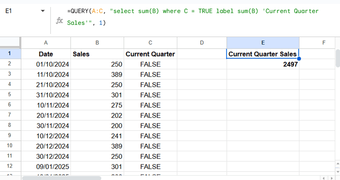
Filter and Summarize Data by Quarter Using QUERY

With your TRUE/FALSE flags in place, you can filter or summarize data effortlessly using QUERY.

For example, suppose you have:

• Dates in A
• Sales in B
• Column C marking TRUE for the current quarter

You can summarize sales for the current quarter with:

=QUERY(A:C, "select sum(B) where C = TRUE label sum(B) 'Current Quarter Sales'", 1)

This automatically returns the total sales for the current quarter — no manual updates needed.

Similarly, you can run the same query on your “Previous Quarter” column for quarter-on-quarter comparisons.

Conclusion

By using dynamic formulas in Google Sheets, you can calculate the current and previous quarter automatically, adapt them to fiscal years, and even mark lists of dates with TRUE/FALSE flags. Combine this with QUERY, and you can filter, summarize, and compare quarterly data without lifting a finger.

With this setup, your reports stay accurate, up to date, and ready for analysis — whether you’re working with calendar years or custom fiscal years.

Related Google Sheets Tutorials

• Extract Quarter from a Date in Google Sheets: Formulas
• Convert Dates to Fiscal Quarters & Years in Google Sheets
• How to Group Dates by Quarter in Google Sheets
• How to Query Non-Calendar Quarters in Google Sheets
• How to Calculate Average by Quarter in Google Sheets