COUNTIF in Google Sheets: A to Z

The COUNTIF function is one of the many functions available in Google Sheets for counting operations. It’s the simplest tool for conditional counting—counting the number of cells that meet specific criteria.

The primary purpose of COUNTIF in Google Sheets is to count how many times a particular value or pattern appears within a range. The function takes two arguments: the range to evaluate and the criteria to apply. These criteria can be a number, text string, or even a formula.

Although COUNTIF is designed for single-condition counts, you can combine it creatively to mimic multiple conditions. For instance, you might use COUNTIF in Google Sheets to count how many cells contain “available” or “in stock”.

In this COUNTIF A to Z tutorial, I’ll cover everything you need to know about using this versatile function: syntax, use with multiple criteria, custom formatting, and more.

Syntax of COUNTIF in Google Sheets

COUNTIF(range, criterion)

To start, type =COUNTIF( in any cell, like A1. Google Sheets will display the function syntax in a helpful tooltip, and clicking on the dropdown will provide additional details.

range: The group of cells you want to test, such as A1:A or A1:C.
criterion: The pattern or condition to match—like "apple", 100, ">"&200, DATE(2023,12,25), or "Joh*".

Dos and Don’ts for COUNTIF Criteria

When using COUNTIF in Google Sheets, keep these things in mind:

For text values, the criterion must be enclosed in double quotes.
You can use wildcard characters in your criteria:
- * (asterisk) = zero or more characters
- ? (question mark) = exactly one character
- ~ (tilde) = escapes a wildcard to treat it as a literal character

For numbers, dates, times, or timestamps, the criterion must match the type of data in the range. If you’re using a comparison operator (like > or <=), enclose it in quotes and concatenate it with the value using &.

COUNTIF with Text

In an attendance sheet where P = Present, A = Absent, and H = Holiday, use:

=COUNTIF(A6:G8, "P")

This counts the number of “P” entries in the range A6:G8. To count “A” values instead, simply change the criterion.

For a dynamic approach, place the condition in a cell (e.g., D2 with “P”) and use:

=COUNTIF(A6:G8, D2)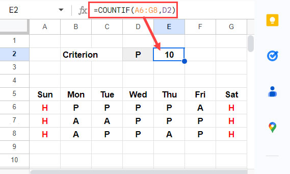

Using COUNTIF formula with a text criterion in Google Sheets

You can also apply COUNTIF to specific rows or columns, like so:

=COUNTIF(E5:E7, "P")

Using Wildcards in COUNTIF in Google Sheets

You can match partial text using wildcards.

Asterisk `*` Examples

=COUNTIF(A2:A, "ID*")    // Starts with "ID"
=COUNTIF(A2:A, "*ID")    // Ends with "ID"
=COUNTIF(A2:A, "*ID*")   // Contains "ID"

Question Mark `?` Examples

=COUNTIF(A2:A, "P??")    // Words that start with "P" and have 2 other characters
=COUNTIF(A2:A, "???")    // Words with exactly 3 characters

Tilde `~` Example

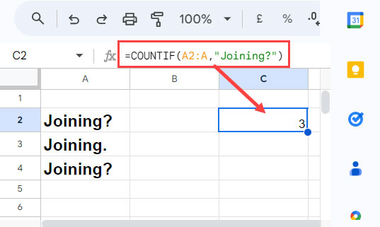
To count exact matches that include a wildcard character:

=COUNTIF(A2:A, "Joining~?")

This matches the literal “Joining?” instead of treating ? as a wildcard.

Using COUNTIF formula with the question mark (?) wildcard in Google Sheets

COUNTIF with Dates, Times, and Timestamps

Dates

=COUNTIF(B2:B15, DATE(2023, 7, 6))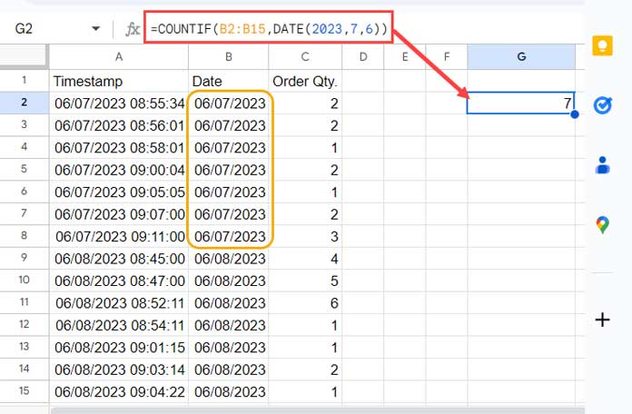

Proper use of a date as a criterion in the COUNTIF formula in Google Sheets

Avoid using ambiguous text dates like “06/07/2023”. Use the DATE() function for accuracy.

For a range:

=COUNTIF(B2:B15, ">="&DATE(2023, 6, 1))

To count calls made today:

=COUNTIF(B2:B15, TODAY())

Time

Use the TIME() function for precision:

=COUNTIF(A2:A, "<"&TIME(9, 30, 0))

Timestamps (Date + Time)

=COUNTIF(A2:A15, ">="&DATE(2023, 7, 6)+TIME(10, 0, 0))

COUNTIF with Numbers

Count cells with specific numbers:

=COUNTIF(C2:C, 0)
=COUNTIF(C2:C, ">"&0)
=COUNTIF(C2:C, "<>"&2)

To count non-blank cells:

=COUNTIF(C2:C, "<>")

If using a cell reference as the criterion, avoid placing the comparison operator in the cell. Instead, include it in the formula:

=COUNTIF(A2:E, ">"&F1)

COUNTIF with Custom Number Formats

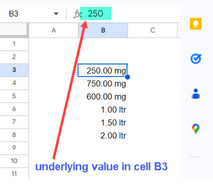
COUNTIF in Google Sheets may not detect units like “mg” or “ltr” added via custom number formatting unless the values are converted to text:

=ARRAYFORMULA(COUNTIF(TO_TEXT(B3:B8), "*ltr"))

Use ARRAYFORMULA because TO_TEXT doesn’t handle ranges on its own.

Displaying the underlying value behind a custom number format in Google Sheets

COUNTIF with Multiple Conditions in Google Sheets

While COUNTIFS is designed for multiple conditions across different ranges, you can still use COUNTIF with multiple conditions in the same range:

=ARRAYFORMULA(COUNTIF(B2:B9, VSTACK(D2, D3)))

This returns two counts—one for each value in D2 and D3.

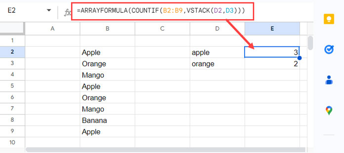
Counting based on multiple conditions using COUNTIF and VSTACK in Google Sheets

For a single total:

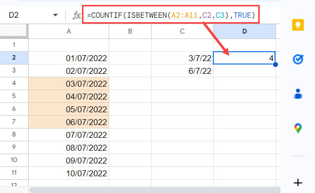
=SUM(ARRAYFORMULA(COUNTIF(B2:B9, VSTACK(D2, D3))))

But when using comparison operators, this trick doesn’t always work. Here’s a workaround using ISBETWEEN:

=COUNTIF(ISBETWEEN(A2:A11, C2, C3), TRUE)

ISBETWEEN checks if each cell in A2:A11 falls between the values in C2 and C3.

COUNTIF formula to count values between two numbers in Google Sheets

Advanced Use: COUNTIF with BYROW and BYCOL

The COUNTIF function in Google Sheets works great with dynamic array functions like BYROW and BYCOL:

To count “x” across a row (e.g., Day 1):

=COUNTIF(B3:E3, "x")

To count “x” in a column (e.g., Week 1):

=COUNTIF(B3:B9, "x")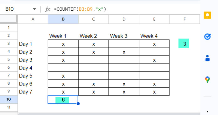

Using COUNTIF with LAMBDA for conditional counting in Google Sheets

When paired with BYROW or BYCOL, COUNTIF in Google Sheets can scale up to evaluate multiple rows or columns at once.

Row-wise count (count “x” in each row):

=BYROW(B3:E9, LAMBDA(val, COUNTIF(val, "x")))

Column-wise count (count “x” in each column):

=BYCOL(B3:E9, LAMBDA(val, COUNTIF(val, "x")))

These formulas return an array of counts—one for each row or column in the specified range.

Conclusion

This concludes the complete tutorial on using COUNTIF in Google Sheets—from the basics to advanced scenarios. Whether you’re working with text, numbers, dates, or even complex dynamic arrays, this function is a reliable tool in your spreadsheet arsenal.

COUNTIF Google Sheets Function: A to Z