There are many scenarios where you may want to count values in each column separately in Google Sheets.

For example, consider an attendance sheet where the first column represents the days, and the corresponding columns represent employee attendance. In this case, you might want to count each employee’s attendance separately.

If each column contains an “x” mark for “Present,” you can simply use the regular COUNTA function. However, if the column contains “Absent” and “Present” entries separately, you might want to apply a conditional count using COUNTIF.

In this situation, I would suggest using the DCOUNTA function, which counts values, including text. You can also apply conditions to include or exclude specific criteria.

The advantage of DCOUNTA over COUNTA and COUNTIF is that it can expand to count values with or without conditions.

Database Requirements for DCOUNTA

The DCOUNTA function requires a header row. If your data doesn’t have a header, you can leave an empty row at the top and include that in the formula to simulate headers.

Example 1: Count Values in Each Column Separately

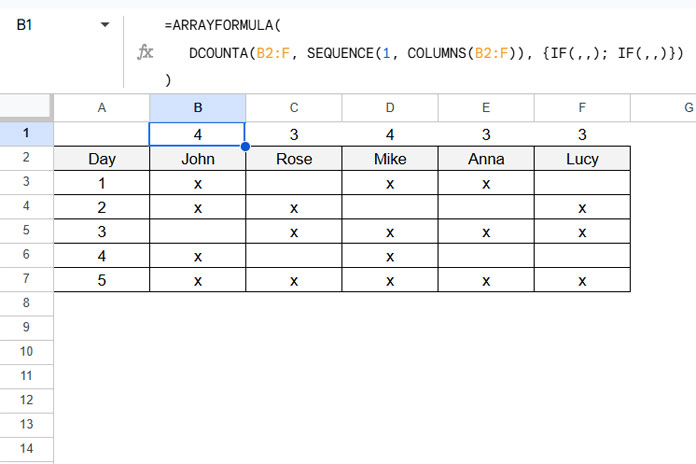
Let’s say you have sample data in the range A2:F, with the headers Days, John, Rose, Mike, Anna, and Lucy. The first column contains sequential numbers from 1 to 5, representing 5 days. The corresponding columns contain “x” marks indicating “Present.”

To count each column separately, use the following formula in cell B1:

=ARRAYFORMULA(
   DCOUNTA(B2:F, SEQUENCE(1, COLUMNS(B2:F)), {IF(,,); IF(,,)})
)

Explanation of the formula:

The syntax of the DCOUNTA function is as follows:

DCOUNTA(database, field, criteria)

Where:

• database: B2:F, the range to count.
• field: SEQUENCE(1, COLUMNS(B2:F)), which generates numbers 1 through 5, corresponding to each column. The SEQUENCE function returns the numbers 1 to 5, based on the COLUMNS(B2:F) (which is 5).
• criteria: {IF(,,); IF(,,)} represents empty criteria, meaning no specific conditions are applied.

If you don’t have a header row and your data starts from B3:F, simply specify the range as B2:F to account for the empty row at the top.

Example 2: Conditional Count Values in Each Column Separately

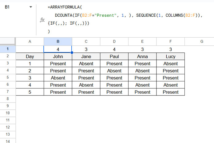
Now, consider the same dataset, but this time the columns contain the text “Present” and “Absent” instead of just “x.”

To count the number of “Present” values for each employee, you can use the DCOUNTA formula with one adjustment:

Instead of the regular ‘database’ range B2:F, use an IF logical statement like IF(B2:F="Present", 1, ). So, the formula will become:

=ARRAYFORMULA(
   DCOUNTA(IF(B2:F="Present", 1, ), SEQUENCE(1, COLUMNS(B2:F)), {IF(,,); IF(,,)})
)

Explanation:

The formula IF(B2:F="Present", 1, ) checks if the cell contains “Present.” If true, it returns 1; otherwise, it returns an empty cell. This way, DCOUNTA counts only the “Present” values.

Additional Options

Instead of using DCOUNTA, you can apply simple formulas directly in each column using the following options:

• Without condition: =COUNTA(B3:B)
• With condition (“Present”): =COUNTIF(B3:B, "Present")

Enter one of these formulas in cell B1, then drag it across to the other columns as per your requirement.

Alternatively, to expand the formulas without dragging, you can use the BYCOL function with a LAMBDA:

• Without condition: =BYCOL(B3:F, LAMBDA(col, COUNTA(col)))
• With condition (“Present”): =BYCOL(B3:F, LAMBDA(col, COUNTIF(col, "Present")))

While LAMBDA functions are powerful, they can be resource-intensive and more complex to understand. For simplicity, I recommend using DCOUNTA to count values in each column separately in Google Sheets.

Conclusion

In this post, we’ve covered how to count values in each column separately in Google Sheets, both with and without conditions. By using functions like DCOUNTA, COUNTIF, and BYCOL, you can easily analyze attendance, inventory, or any other data organized in columns.

Resources

• Count a Column with Multiple Conditions in Google Sheets
• Countif Across Columns Row by Row – Array Formula in Google Sheets
• OR Logic in Multiple Columns with COUNTIFS in Google Sheets
• OR Logic in COUNTIFS Across Either Column in Google Sheets
• Counting Unique Values in Multiple Columns in Google Sheets
• How to Count Duplicate Values in a Column in Google Sheets