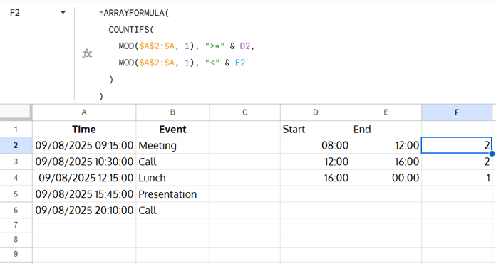
Count Events by Timeslot in Google Sheets

If you’ve ever worked with timestamped data in Google Sheets, you may have needed to figure out how many events occur within certain time ranges — for example, morning vs afternoon vs evening. In this guide, we’ll show you 4 easy methods to Count Events by Timeslot in Google Sheets, covering both beginner-friendly formulas and advanced options.

We’ll explore:

COUNTIFS (straightforward, built-in conditional count)
SUMPRODUCT (flexible, clean logic)
FILTER + COUNT (simple to read)
QUERY (powerful, for advanced users)

By the end, you’ll know exactly how to handle time range counting for any dataset.

Table of Contents

Understanding the Scenario

Let’s say you have the following data in A1:B:

Time	Event
09/08/2025 09:15:00	Meeting
09/08/2025 10:30:00	Call
09/08/2025 12:15:00	Lunch
09/08/2025 15:45:00	Presentation
09/08/2025 20:10:00	Call

You want to count how many of these events occur in specific time slots, such as:

08:00–12:00 → Morning
12:00–16:00 → Afternoon
16:00–00:00 → Evening

Sample Data & Timeslot Setup

We’ll keep the event data in columns A and B and place our timeslot ranges in columns D and E:

Start Time	End Time
08:00	12:00
12:00	16:00
16:00	24:00

Tip: For a timeslot that ends at midnight, enter the end time as 24:00 (end of day) rather than 00:00. Google Sheets stores 24:00 as the serial value 1 (a full day). How the cell displays depends on its number format: some formats show 24:00:00, while HH:MM-style formats display 00:00 because hours are shown modulo 24. Either way the underlying value is the end-of-day.

1. COUNTIFS — Easiest Way to Count Events by Timeslot in Google Sheets

COUNTIFS is the most straightforward function for this job.

Formula in F2:

=ARRAYFORMULA(
  COUNTIFS(
    MOD($A$2:$A, 1), ">=" & D2,
    MOD($A$2:$A, 1), "<" & E2
  )
)

Then drag down for other rows.

Google Sheets example showing how to count events in particular timeslots using COUNTIFS formula

How it works:

MOD($A$2:$A, 1) extracts just the time portion from each timestamp.
The two criteria check if the time falls between the start and end values in columns D and E.
< E2 makes the end time exclusive, so there’s no overlap between slots.

2. SUMPRODUCT — Cleaner Logic Without COUNTIFS

SUMPRODUCT can often be cleaner because it handles arrays naturally without ARRAYFORMULA.

Formula in F2:

=SUMPRODUCT(
  (MOD($A$2:$A, 1) >= D2) *
  (MOD($A$2:$A, 1) < E2)
)

How it works:

Each condition returns an array of TRUE/FALSE values (which become 1/0).
Multiplying the arrays means only rows matching both conditions become 1.
SUMPRODUCT then sums these up to give the count.

3. FILTER + COUNT — Readable Step-by-Step Method

This approach uses FILTER to grab only matching rows, then counts them.

Formula in F2:

=COUNT(
  FILTER(
    $A$2:$A,
    MOD($A$2:$A, 1) >= D2,
    MOD($A$2:$A, 1) < E2
  )
)

How it works:

FILTER pulls only the event times that fall within the current slot.
COUNT returns how many were found.

This method is highly readable and great for beginners.

4. QUERY — Advanced Count Events by Timeslot in Google Sheets

QUERY lets you write SQL-like conditions directly. It’s more complex but very powerful.

Formula in F2:

=ARRAYFORMULA(
  QUERY(
    {MOD(TOCOL($A$2:$A, 3), 1)},
    "SELECT COUNT(Col1) 
     WHERE Col1 >= TIMEOFDAY '" & TEXT(D2, "HH:MM:SS") & "' 
     AND Col1 < TIMEOFDAY '" & IF(TIMEVALUE(E2)=0, "24:00:00", TEXT(E2, "HH:MM:SS")) & "' 
     LABEL COUNT(Col1) ''",
    0
  )
)

How it works:

MOD(TOCOL(...), 1) extracts the time portion of each date-time value, while TOCOL removes any empty or error cells from the column.
TIMEOFDAY is used in the query to compare times.
IF(TIMEVALUE(E2)=0, "24:00:00", ...) fixes the midnight issue by treating 00:00 as end-of-day.
LABEL COUNT(Col1) '' removes the default column label.

Comparison of Methods to Count Events by Timeslot in Google Sheets

Method	Difficulty	Handles Midnight Easily	Best For
COUNTIFS	Easy	Needs 24:00 trick	Beginners
SUMPRODUCT	Medium	Needs 24:00 trick	Clean formulas
FILTER + COUNT	Easy	Needs 24:00 trick	Readability
QUERY	Advanced	Yes (in formula)	Complex queries

Conclusion

You now have four different ways to Count Events by Timeslot in Google Sheets.

For quick tasks, COUNTIFS or FILTER are easiest.
For more flexibility, SUMPRODUCT keeps formulas tidy.
For advanced scenarios, QUERY offers unmatched control.

Want a simpler, COUNTIFS-only solution? Check out our step-by-step guide: How to Use COUNTIFS with Time Ranges in Google Sheets.