


")


")

")
")
 in Excel & Google Sheets")


This tutorial offers a powerful formula-based solution to count consecutive workday absences in Google Sheets. It intelligently excludes weekends (e.g., Saturday and Sunday) and optionally specified holidays.
You’ll learn how to:
- Identify uninterrupted streaks of workday absences for each employee
- Return only those periods that span two or more workdays
- Easily customize for different weekend settings and holiday calendars
- Track multiple employees’ sick leave patterns at once
Why Count Consecutive Workday Absences?
Tracking only the total number of absences isn’t always helpful. HR teams, operations, and team leads often need to assess continuous absences, especially when:
- An employee’s leave policy changes after a certain number of days (e.g., requiring a doctor’s note)
- Project timelines need to be updated based on prolonged unavailability
- Shift scheduling depends on knowing how long someone will be out
This formula goes beyond basic counting and delivers accurate absence streaks, even when spread across a month or year.
Who Will Benefit?
- HR Professionals: Ensure compliance with company policies on sick leave, especially when employees exceed a certain number of consecutive days.
- Team Leaders: Adjust workloads and timelines by identifying continuous periods of unavailability.
- Operations Managers: Ensure adequate coverage by forecasting consecutive leave periods for multiple staff members at once.
You can follow along using this sample Google Sheet. It includes employee names, absence start and end dates, and a holiday list.
Sample Dataset
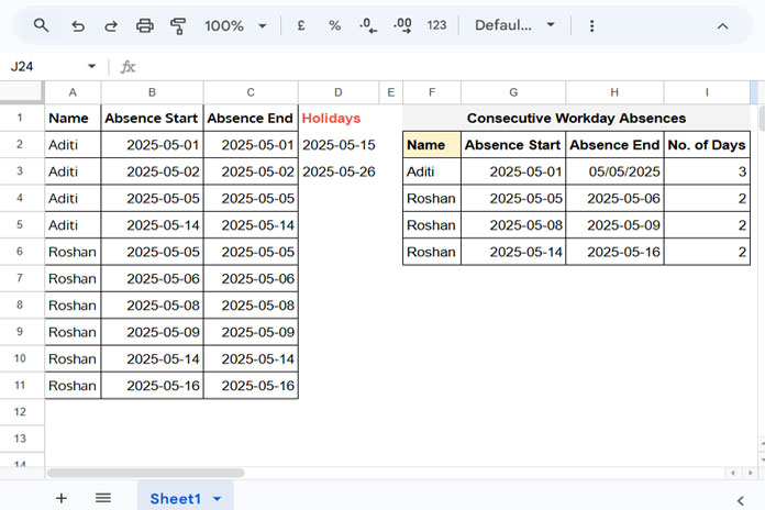
Here’s an example of how your data might be structured:
| Name | Absence Start | Absence End |
| Aditi | 2025-05-01 | 2025-05-01 |
| Aditi | 2025-05-02 | 2025-05-02 |
| Aditi | 2025-05-05 | 2025-05-05 |
| Aditi | 2025-05-14 | 2025-05-14 |
| Roshan | 2025-05-05 | 2025-05-05 |
| Roshan | 2025-05-06 | 2025-05-06 |
| Roshan | 2025-05-08 | 2025-05-08 |
| Roshan | 2025-05-09 | 2025-05-09 |
| Roshan | 2025-05-14 | 2025-05-14 |
Notes:
- Each row here reflects a single workday of absence.
- You can also use a single row per absence period (e.g., from
2025-05-01to2025-05-10)—the formula supports both structures. - The formula works for one or many employees.
Goal
We want to output a summarized report like this:
| Name | Absence Start | Absence End | No. of Days |
| Aditi | 2025-05-01 | 2025-05-05 | 3 |
| Roshan | 2025-05-05 | 2025-05-06 | 2 |
| Roshan | 2025-05-08 | 2025-05-09 | 2 |
This lets you count consecutive workday absences while ignoring weekends and optional holidays.
- Weekends and holidays DO NOT break the continuity of an absence streak.
- If an employee is absent before and after a weekend or holiday, the absence is still considered consecutive.
- The Absence Start and Absence End dates represent the true span of each streak — including any intervening weekends or holidays.
- The No. of Days column counts only the working days (excludes weekends and holidays), using the
NETWORKDAYS.INTLfunction.
Let’s say an employee, Aditi, has absence records on:
- 2025-05-01 (Thursday)
- 2025-05-02 (Friday)
- 2025-05-05 (Monday)
Even though May 3–4 (Saturday and Sunday) fall between these dates, the absence streak is still considered continuous.
So the output will be:
| Name | Absence Start | Absence End | No. of Days |
| Aditi | 2025-05-01 | 2025-05-05 | 3 |
Absence Start: 2025-05-01Absence End: 2025-05-05No. of Days: 3 (excluding Sat-Sun using"0000011").
If you want to count all days including weekends, such that the total becomes 5 instead of 3, I’ll explain how to adjust the formula after the main formula section.
The Formula: Count Consecutive Workday Absences in Google Sheets
Paste the following formula into a cell:
=LET(cabsence, ARRAYFORMULA(REDUCE(TOCOL(,3), TOCOL(UNIQUE(A2:A), 3), LAMBDA(acc, name, VSTACK(acc,
   IFNA(
      HSTACK(
         name,
         LET(
            raw_data, VSTACK(FILTER(HSTACK(ROW(B2:B), B2:B), A2:A=name), FILTER(HSTACK(ROW(C2:C), C2:C), A2:A=name)),
            process, UNIQUE(SORT(raw_data, 2, 1)),
            pcolA, CHOOSECOLS(process, 1),
            pcolB, CHOOSECOLS(process, 2),
            end,
               TOCOL(
                  MAP(SEQUENCE(ROWS(pcolB), 1, 2), LAMBDA(seq, LET(capture, LAMBDA(col, INDEX(col, seq-1)),
                  colA, capture(pcolA), colB, capture(pcolB),
                  IF(OR(INDEX(pcolB, seq)=WORKDAY.INTL(colB, 1, "0000011", TOCOL(D2:D, 3)), INDEX(pcolA, seq)=colA),,colB)))), 3
               ),
            start, XLOOKUP(end+1, pcolB, pcolB, ,1),
            dts, SORT(VSTACK(start, end, MIN(pcolB), MAX(pcolB))),
            format, WRAPROWS(dts, 2),
            fnl, NETWORKDAYS.INTL(CHOOSECOLS(format, 1), CHOOSECOLS(format, 2), "0000011", TOCOL(D2:D, 3)),
            HSTACK(format, fnl)
        )
      ), name
   )
)))), VSTACK(HSTACK("Name", "Absence Start", "Absence End", "No. of Days"), FILTER(cabsence, CHOOSECOLS(cabsence, 4)>1)))
You’ll notice that the formula returns date values in the result columns for consecutive absence start and end dates. To display them correctly, select those columns and go to Format > Number > Date.
Input Columns
- A2:A → Employee Name or ID
- B2:B → Absence Start Date
- C2:C → Absence End Date
- D2:D → List of holidays (optional)
- “0000011” → Weekends specified as Saturday and Sunday
Note: You can specify weekends in the formula using a 7-digit string of 0s and 1s, where the first digit represents Monday and the last digit represents Sunday.
A 0 indicates a workday, and a 1 indicates a weekend.
So, “0000011” means Saturday and Sunday are weekends.
Optional Behavior: If You Truly Want to Include Weekends in the Day Count
If, for some use cases, you want the number of calendar days (including weekends), you can tweak this part of the formula:
Replace:
NETWORKDAYS.INTL(CHOOSECOLS(format, 1), CHOOSECOLS(format, 2), "0000011", TOCOL(D2:D, 3))With:
NETWORKDAYS.INTL(CHOOSECOLS(format, 1), CHOOSECOLS(format, 2), "0000000")But note: This will count every day, including Saturdays, Sundays, and holidays.
Formula Explanation
Here are the key components of the formula. This will help you understand how the formula counts Consecutive Workday Absences in Google Sheets.
1. raw_data
VSTACK(FILTER(HSTACK(ROW(B2:B), B2:B), A2:A=name), FILTER(HSTACK(ROW(C2:C), C2:C), A2:A=name))- Creates a two-column array
{row_number, date}for the selected employee (name). - First part collects row numbers and Absence Start dates.
- Second part collects row numbers and Absence End dates.
- Both are stacked vertically using
VSTACK.
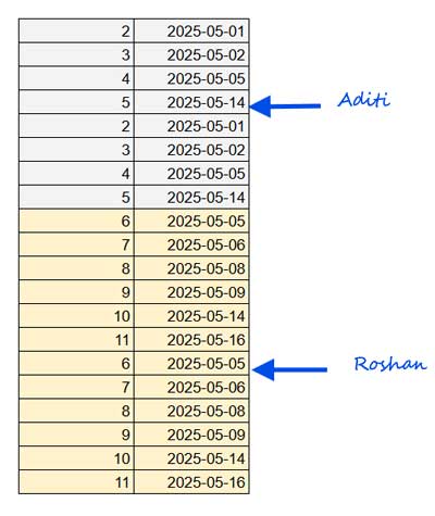
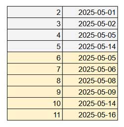
2. process
UNIQUE(SORT(raw_data, 2, 1))- Sorts the stacked array by the date column (column 2).
- Removes duplicate entries.
For example:
{2, 2025-05-01} // Absence Start
{2, 2025-05-01} // Absence End
The duplicate {2, 2025-05-01} is removed.
3. end
TOCOL(
   MAP(SEQUENCE(ROWS(pcolB), 1, 2), LAMBDA(seq, LET(capture, LAMBDA(col, INDEX(col, seq-1)),
   colA, capture(pcolA), colB, capture(pcolB),
   IF(OR(INDEX(pcolB, seq)=WORKDAY.INTL(colB, 1, "0000011", TOCOL(D2:D, 3)), INDEX(pcolA, seq)=colA),,colB)))), 3
)- Identifies where each consecutive absence streak ends.
- Checks whether two dates in sequence are consecutive workdays (excluding weekends/holidays).
- Returns the date where the streak ends.
4. start
XLOOKUP(end+1, pcolB, pcolB, ,1)- Finds the start of each absence streak by looking up the next workday after the end date.
- Uses the sorted list (
pcolB, i.e.,CHOOSECOLS(process, 2)) to identify where each streak begins.
5. dts
SORT(VSTACK(start, end, MIN(pcolB), MAX(pcolB)))- Stacks:
- All calculated start and end dates,
- The first and last dates from
pcolB(in case they’re missed),
- Then sorts the list to get a clean date sequence.
6. format
WRAPROWS(dts, 2)- Converts the sorted list into a two-column table:
- Column 1 = absence start
- Column 2 = absence end
7. fnl
NETWORKDAYS.INTL(CHOOSECOLS(format, 1), CHOOSECOLS(format, 2), "0000011", TOCOL(D2:D, 3))- Counts the number of working days between each absence start and end date.
- Weekends and provided holidays are excluded from the count.
Final Output:
- Use
HSTACKto combine the start, end, and count into a single result array. - The entire logic is applied individually for each employee.
- The result filters out any single-day absences where the working days count is 1 or less.
Error Handling Tips
- If your formula returns incorrect streaks, check for overlapping absence entries. For example:
Start: 2025-05-01,End: 2025-05-10- Another entry:
2025-05-06will break the logic.
- For large datasets:
- Remove blank rows in your source data
- Limit your range (e.g., A2:A1000 instead of full columns)
- Consider applying the formula per employee if performance drops
Related Resources
To deepen your understanding and extend this logic: