Compare All Columns with Each Other for Duplicates in Google Sheets

It’s not easy to compare all columns, with each other, for duplicates in Google Sheets. It’s because there is no function available for this.

So I’ve coded a custom-named function and a child function for this. They are COMPARE_ALL_COLUMNS and CAC_CHILD.

Other than this, you will get the formulas-based approaches also for this.

The custom-named function will return the duplicates in columns, whereas the child function, the columns in comparison.

What input should we give to the formula to compare all columns and return duplicates?

You feed only the range reference, for example, A2:C7.

The comparison will be between A2:A7 & B2:B7, A2:A7 & C2:C7, and B2:B7 & C2:C7.

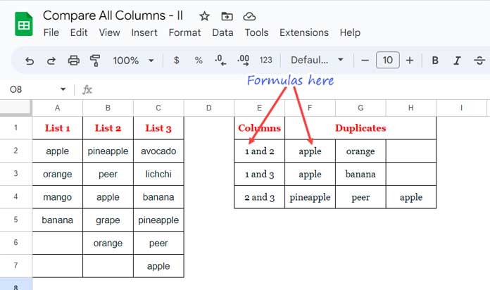
Compare All Columns with Each Other for Duplicates - E.g. 1
example # 1

In the above example, the child function returns the values in E2:E4, and the main one the duplicates, i.e., common fruit names, in F2:H4.

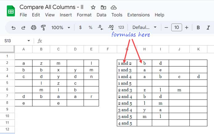
Here is one more example to compare or match all columns with each other and return the duplicates in Google Sheets.

This time there are five columns to compare.

Range: A2:E8
Child Formula: G2
Master Formula: H2

Compare All Columns with Each Other for Duplicates - E.g. 2
example # 2

Using these functions in real-life, you can check whether the same names are included in multiple teams.

COMPARE_ALL_COLUMNS and CAC_CHILD: Syntax and Arguments

Syntax: COMPARE_ALL_COLUMNS(range)

ArgumentDescription
rangeThe range of columns to compare with each other and return duplicates.
It can be a range reference like A2:C100 or an array {A2:A100, B2:B100, C2:C100}. So you can include distant columns to compare.

Syntax: CAC_CHILD(range)

ArgumentDescription
rangeThe column range.
It can also be a range reference like A2:C100 or an array {A2:A100, B2:B100, C2:C100}.

You can import these functions from my sample Sheet below and use them straightaway to compare all columns with each other for finding common values.

Functions 9323

Instructions to Import

Use the above button to make a copy of my Sheet that contains those two functions.

Open the Sheet in which you want to use them. In that Sheet, go to Data > Named functions > Import function.

Follow the onscreen instructions, and voila!

You are ready to use my above two named functions to compare all columns (lists) in a given range and return the duplicate/common values.

Compare All Columns with Each Other for Duplicates Named Functions

I’ve given two examples at the beginning of this tutorial.

The first one contains fruit names in A2:C7. Here are the formulas in use in E2 and F2.

E2 (Child Function):

=CAC_CHILD(A2:C7)

F2 (Main Function):

=COMPARE_ALL_COLUMNS(A2:C7)

Please note that we can include distant columns in these named functions providing them as an array like {A2:A7, F2:F7, Z2:Z7} in range.

The E2 formula returns the columns in comparison.

The role of the F2 formula is to compare all columns with each other and return the matching/duplicate values.

Can we use an open range like A2:C instead of A2:A7?

Yes. But I advise using closed ranges to improve the performance of functions in Google Sheets.

In the second example, we have compared values in columns A2:E8. But I have used an open range.

G2:

=CAC_CHILD(A2:E)

H2:

=COMPARE_ALL_COLUMNS(A2:E)

I hope the above examples are enough to understand the usage of the custom functions COMPARE_ALL_COLUMNS and CAC_CHILD.

Compare All Columns with Each Other for Duplicates — Formulas

Some of you may not want to import and use my custom functions for this. If so, you can use the following formulas.

The following is equivalent to the child function, i.e., CAC_CHILD.

=ArrayFormula(lambda(range,sort(let(setA,flatten(makearray(columns(range)-1,columns(range)-1,lambda(r,c,r+c))),setB,flatten(makearray(columns(range)-1,columns(range)-1,lambda(r,c,c))),filter(setB,setA<=columns(range))))&" and "&let(setA,flatten(makearray(columns(range)-1,columns(range)-1,lambda(r,c,r+c))),filter(setA,setA<=columns(range))))(A2:E))

Replace A2:E with your actual range.

What about the COMPARE_ALL_COLUMNS equivalent?

Here you go!

=lambda(range,map(sort(let(setA,flatten(makearray(columns(range)-1,columns(range)-1,lambda(r,c,r+c))),setB,flatten(makearray(columns(range)-1,columns(range)-1,lambda(r,c,c))),filter(setB,setA<=columns(range)))),let(setA,flatten(makearray(columns(range)-1,columns(range)-1,lambda(r,c,r+c))),filter(setA,setA<=columns(range))),lambda(two,one, transpose(ifna(unique(filter(index(range,0,two),xmatch(index(range,0,two),index(range,0,one),0))))))))(A2:E)

Here also replace A2:E with your actual range.

We can easily use these formulas to compare/match all columns with each other for duplicates because of the LAMBDA use.

The LAMBDA and LET functions help us use the range reference only once in the formula.

So easy for anyone to adapt the formula in their Sheet.

If you are a Google Sheets enthusiast, you might want to know the logic behind the above formulas.

To be frank, I’ve coded both of them based on the same logic, and here it is.

Anatomy of the Formulas

Assume there are five teams with seven players each.

We can call the teams by the numbers 1, 2, 3, 4, and 5.

If you want to check whether any player in Team # 1 is present in any other teams, you can use BYCOL with FILTER and XLOOKUP or COUNTIF for that.

The matching would be between columns 1 & 2, 1 & 3, and 1 & 4.

But what about matching all teams with each other to find repeating names?

The matching must be like this:

Columns to MatchMatch With
12
13
14
15
23
24
25
34
35
45

If we can generate these two sets of numbers, we can use the INDEX function to offset the range accordingly and compare all columns with each other.

My thought process was around this logic. I could find a solution using the MAKEARRAY function.

There are three steps each for generating the above two lists of numbers.

Let’s start with “Match With” first.

“Match With” Part

Returns a 4 x 4 matrix (Step # 1 A).

=makearray(columns(A2:E)-1,columns(A2:E)-1,lambda(r,c,r+c))

Flatten Step # 1 A result (Step # 1 B).

=flatten(makearray(columns(A2:E)-1,columns(A2:E)-1,lambda(r,c,r+c)))

Filter out values greater than 5 (total columns in the range) from Step # 1 B result (Step # 1 C).

=lambda(n_c,let(setA,flatten(makearray(n_c-1,n_c-1,lambda(r,c,r+c))),filter(setA,setA<=n_c)))(5)
The Role of MAKEARRAY (Anatomy of the Formula)

“Columns to Match” Part

Returns a 4 x 4 matrix (Step # 2 A).

=lambda(n_c,makearray(n_c-1,n_c-1,lambda(r,c,c)))(5)

Flatten Step # 2 A result (Step # 2 B).

=lambda(n_c,flatten(makearray(n_c-1,n_c-1,lambda(r,c,c))))(5)

Filter out Step # 2 B values if Step # 1 B values are >5 (Step # 2 C).

=lambda(n_c,sort(let(setA,flatten(makearray(columns(A2:E)-1,columns(A2:E)-1,lambda(r,c,r+c))),setB,flatten(makearray(n_c-1,n_c-1,lambda(r,c,c))),filter(setB,setA<=n_c))))(5)

The final formula uses the above two lists of generated numbers to compare all columns with each other for duplicates.

Please scroll up and see my sample Sheet to learn the above steps physically and how to use them to compare all columns with each other and return the common names/values.

Prashanth KV
Prashanth KV
Your Trusted Google Sheets and Excel Guide Prashanth KV brings a wealth of experience in Google Sheets and Excel, cultivated through years of work with multinational corporations in Mumbai and Dubai. As a recognized Google Product Expert in Docs Editors, Prashanth shares his expertise through insightful blogging since 2012. Explore his blog for practical tips and guidance on maximizing your spreadsheet skills.

Highlight Upcoming Birthdays in Google Sheets

When highlighting upcoming birthdays in Google Sheets, one important aspect is ignoring the year...

Compare Two Tables for Differences in Excel

To compare two tables with similar data for differences, you can use the XLOOKUP...

Calculate Weighted Average in Pivot Table in Google Sheets

You can calculate a weighted average in a Pivot Table using a custom formula...

Summarize Data and Keep the Last Record in Google Sheets

In Google Sheets, we can summarize data (like sum, average, min, max, count) using...

More like this

Highlight Upcoming Birthdays in Google Sheets

When highlighting upcoming birthdays in Google Sheets, one important aspect is ignoring the year...

Calculate Weighted Average in Pivot Table in Google Sheets

You can calculate a weighted average in a Pivot Table using a custom formula...

Summarize Data and Keep the Last Record in Google Sheets

In Google Sheets, we can summarize data (like sum, average, min, max, count) using...

LEAVE A REPLY

Please enter your comment!
Please enter your name here

This site uses Akismet to reduce spam. Learn how your comment data is processed.