


")


")

")
")
 in Excel & Google Sheets")


In Google Sheets, duplicate rows may contain partial or updated information for the same entity. Manually consolidating these records can be time-consuming and error-prone. In such cases, you may need to combine rows and keep the latest values for each entry—ensuring that your data remains accurate and up to date. Doing this manually can be tedious and lead to wasted time. Fortunately, you can automate this process using a powerful formula.
For example, in an HR database, employees may update their contact details over time, but not all fields are filled in with every update.
By combining duplicate rows and retaining the most recent values, you can create a clean, consolidated record without losing important data.
Example Scenario
Assume you have the following records of an employee:
| Employee ID | Name | Phone | Department | Updated Date | |
| 1000 | Winnie | winnie_95@example.com | 123-456-2501 | HR | 10/02/2024 |
| 1000 | Winnie | 987-654-1234 | 15/02/2024 |
If the formula removes duplicates based on Employee ID and retains the latest record, you will get the following result:
| Employee ID | Name | Phone | Department | Updated Date | |
| 1000 | Winnie | winnie_95@example.com | 987-654-1234 | HR | 15/02/2024 |
In this tutorial, you’ll learn how to efficiently combine rows and keep the latest values in Google Sheets using a formula—without relying on scripts or add-ons. Let’s get started!
👉 Copy Example Google Sheet to follow along with this tutorial.
Generic Formula
=IFNA(BYCOL(data, LAMBDA(col, MAP(UNIQUE(id_column), LAMBDA(roww, XLOOKUP(roww, FILTER(id_column, id_column=roww, col<>""), TOCOL(FILTER(col, id_column=roww), 1), ,0,-1))))))Usage: Replace data with your actual data range and id_column with the column containing unique identifiers in your dataset.
Example: Combining Rows and Keeping the Latest Values in Google Sheets
Here is a sample employee dataset that you can work with, located in Sheet1 (range A1:F).
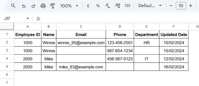
Steps to Apply the Formula:
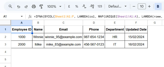
- In Sheet2, enter the following formula in cell A1:
=IFNA(BYCOL(Sheet1!A1:F, LAMBDA(col, MAP(UNIQUE(Sheet1!A1:A), LAMBDA(roww, XLOOKUP(roww, FILTER(Sheet1!A1:A, Sheet1!A1:A=roww, col<>""), TOCOL(FILTER(col, Sheet1!A1:A=roww), 1), ,0,-1))))))- Press Enter, and the formula will automatically combine duplicate rows while keeping the latest values.
Handling Date Columns:
If your dataset contains a date or datetime column, the formula may return numeric date values. To fix this:
- Select the column.
- Go to Format > Number > Date or Datetime to display the correct format.
Explanation of Formula Components
Some of you might want to understand how the formula works. Here is a breakdown of each component:
Sheet1!A1:F– The data range.Sheet1!A1:A– The unique ID column, used to identify duplicates.UNIQUE(Sheet1!A1:A)– Extracts unique employee IDs.FILTER(Sheet1!A1:A, Sheet1!A1:A=roww, col<>"")– Filters column A for the current employee ID (roww), excluding empty values.TOCOL(FILTER(col, Sheet1!A1:A=roww), 1)– Filters each column for the current employee ID and removes blanks.XLOOKUP(roww, FILTER(Sheet1!A1:A, Sheet1!A1:A=roww, col<>""), TOCOL(FILTER(col, Sheet1!A1:A=roww), 1), ,0,-1)– Searches for the employee ID and retrieves the latest (last) non-blank value from the column.- MAP – Applies the function to each unique employee ID.
- BYCOL – Ensures the formula is executed separately for each column.
This formula allows you to combine duplicate rows and keep the latest values dynamically.
Why is This Useful?
This dynamic approach helps keep your data concise and up-to-date without manual intervention. It ensures that you always retrieve the latest information for reports, dashboards, or further processing.
This method is particularly useful in various applications, such as:
- HR records – Consolidating employee updates.
- Inventory management – Maintaining the most recent stock information.
- Financial records – Ensuring only the latest transactions are retained.