To create a case-sensitive pivot table in Google Sheets, we will use a helper formula. This formula generates a helper column to assist in grouping data case-sensitively.
Why You Need a Case-Sensitive Pivot Table
The Pivot Table in Google Sheets is case-insensitive by default. This can cause issues when working with case-sensitive data, such as usernames, codes, or identifiers, which play a critical role in certain datasets.
For example, imagine you have a dataset of customer IDs and their purchase details. Some customer IDs are entered with varying cases, such as “AB001,” “ab001,” and “Ab001.” These entries represent different customers. However, when creating a pivot table in Google Sheets to summarize purchase data, such as total sales per customer ID, a standard pivot table will treat all variations of these IDs as the same entity.
If you want to analyze the data for each unique case variation, you can use the following helper formula:
=ARRAYFORMULA(
   LET(
      range, A2:A,
      uniq, TOCOL(UNIQUE(range), 1),
      rc, COUNTIFS(uniq, uniq, SEQUENCE(ROWS(uniq)), "<="&SEQUENCE(ROWS(uniq))),
      lup, MAP(range, LAMBDA(r, XLOOKUP(TRUE, EXACT(r, uniq), rc))),
      fnl, IF(range="",,range&" ("&lup&")"),
      VSTACK("Customer ID", fnl)
   )
)
Replace A2:A with the range containing your customer IDs, and replace "Customer ID" with the field label of the range (the value in cell A1). Then, enter the formula in an empty column next to your data.
This formula allows you to create a case-sensitive pivot table where case-sensitive data, such as usernames, codes, or identifiers, is crucial. Let’s walk through an example.
This tutorial is part of the Pivot Table Calculations & Advanced Metrics hub, covering advanced pivot table calculations in Google Sheets.
1. Sample Data
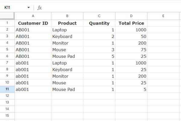
Here’s an example dataset:

The range is A1:D, with A1:D1 containing the field labels.
2. Helper Formula for Case-Sensitive Grouping
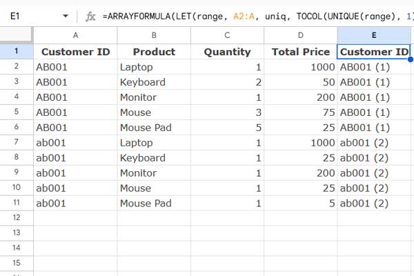
Enter the above formula in cell E1. The helper column will generate distinct values by appending a number to each duplicate entry based on its case sensitivity. Use this column instead of column A when creating the pivot table.

3. Creating a Case-Sensitive Pivot Table
Follow these steps to create the case-sensitive pivot table:
- Select the range
B1:E, excluding the first column (A), but including the new helper column (E). - Click Insert > Pivot Table.
- In the dialog box that appears, click Create. This will create a new sheet with the pivot table layout.
- Drag and drop the helper column (e.g., “Customer ID”) under Rows.
- Drag and drop the Total Price field under Values.
- (Optional) Add filters:
- Drag and drop the “Customer ID” field under Filters.
- Use the filter dropdown to exclude empty values by selecting Filter by Condition > Is Not Empty.
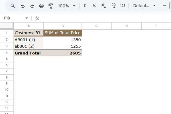
This will create a case-sensitive pivot table grouped by customer IDs.

4. Creating a Case-Sensitive Pivot Table with Multiple Fields
If you want to group by additional fields, such as “Category” or “Product,” you can drag and drop those fields under Rows or Columns.
Usually, secondary fields like “Category” may not require case sensitivity. However, if case sensitivity is needed for another column, create a new helper column for that field using the same formula, replacing A2:A with the relevant range. Use this new column for grouping instead of the original column.
Formula Breakdown
Here’s a detailed breakdown of the helper formula:
TOCOL(UNIQUE(range), 1)— Extracts distinct values and removes empty cells. (Note: UNIQUE is case-sensitive in Google Sheets.) This result is nameduniqusing LET.COUNTIFS(uniq, uniq, SEQUENCE(ROWS(uniq)), "<="&SEQUENCE(ROWS(uniq)))— Returns a running count of distinct items inuniq. This result is namedrc.
These two steps will return the following, where the first column contains uniq and the second column contains rc:
| uniq | rc |
| AB001 | 1 |
| ab001 | 2 |
MAP(range, LAMBDA(r, XLOOKUP(TRUE, EXACT(r, uniq), rc)))— Uses XLOOKUP to perform a case-sensitive search ofrange, i.e., A2:A, inuniqand returns values fromrc. This result is namedlup. XLOOKUP is not case-sensitive, so we used EXACT with it. Related: Case-Sensitive VLOOKUP in Google Sheets.
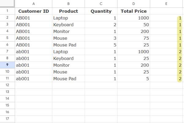
Here is the result against the range:

IF(A2:A="",,A2:A&" ("&lup&")")— Combines the original data (A2:A) withlupto generate distinct case-sensitive values. This result is namedfnl.VSTACK("Customer ID", fnl)— Adds the field label to the result offnl.
Conclusion
By using the helper formula and following these steps, you can create a case-sensitive pivot table in Google Sheets. This approach ensures accurate analysis of case-sensitive data, such as usernames, codes, or identifiers.


