


")


")

")
")
 in Excel & Google Sheets")


For a case-sensitive COUNTIF, you may need to use REGEXMATCH or EXACT in conjunction with the COUNTIF function in Google Sheets. Alternatively, you can use a QUERY.
Sometimes, the interpretation of values differs based on their case. For example, “COMPLETED” might represent the completion of a job that took a significant amount of time, while “Completed” could indicate a regular completion.
If you have a list containing several values and want to count a value case-sensitively, the following tips may be useful.
Case-Sensitive COUNTIF in Google Sheets: An Example
In the following example, I have a list in B3:B, and I want to count the occurrence of “COMPLETED” in this list case-sensitively.
A regular COUNTIF would return an inaccurate count since it is case-insensitive:
=COUNTIF(B3:B, "COMPLETED")In this formula, B3:B is the range, and “COMPLETED” is the criterion.
Syntax: COUNTIF(range, criterion)
To perform a case-sensitive count, we can use REGEXMATCH or EXACT to match the criterion in the range, returning an array of TRUE or FALSE values, where TRUE indicates an exact case-sensitive match.
Use that array as the range in COUNTIF, with TRUE as the criterion to count:
=ArrayFormula(COUNTIF(EXACT(B3:B,"COMPLETED"), TRUE))
=ArrayFormula(COUNTIF(REGEXMATCH(B3:B, "^COMPLETED$"), TRUE))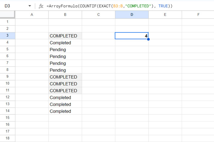
These two formulas are examples of how to perform a case-sensitive COUNTIF in Google Sheets.
Notes:
- Both EXACT and REGEXMATCH are non-array functions, so you must use ARRAYFORMULA with them when referring to a range.
- In REGEXMATCH, the caret (^) at the beginning and the dollar sign ($) at the end of the criterion ensure an exact match.
Case-Sensitive Count Using the QUERY Function
You can use the following QUERY formula as an alternative to a case-sensitive COUNTIF formula in Google Sheets:
=QUERY({B3:B}, "SELECT COUNT(Col1) WHERE Col1='COMPLETED' LABEL COUNT(Col1)''")Don’t worry about the complexity of the formula. Simply replace B3:B with the range containing the values to count and ‘COMPLETED’ with your criterion. The formula will handle the rest.
Bottom Line
For case-sensitive COUNTIF, there are mainly three approaches in Google Sheets:
- COUNTIF and EXACT Combo
- COUNTIF and REGEXMATCH Combo
- QUERY
You may encounter different variations of these methods. For example, you can replace COUNTIF with SUM as follows:
=ArrayFormula(SUM(--EXACT(B3:B,"COMPLETED")))This approach is also applicable to formulas using REGEXMATCH because both REGEXMATCH and EXACT return an array of TRUE or FALSE, where TRUE is converted to 1 and FALSE to 0.
To facilitate the summation, the -- unary operator is used to convert boolean values into numbers.
Another option is to use SUMPRODUCT:
=SUMPRODUCT(EXACT(B3:B,"COMPLETED"))
=SUMPRODUCT(REGEXMATCH(B3:B, "^COMPLETED$"))
In this case, there is no need to convert boolean values to numbers, and ARRAYFORMULA is not required because SUMPRODUCT is already an array function.
For case-sensitive COUNTIF, which is the best function in Google Sheets?
I would suggest using the COUNTIF and EXACT combo for its simplicity. If you need more flexibility, such as partial matches, you can use either QUERY or COUNTIF with REGEXMATCH. However, you may need to understand these functions better. Additionally, QUERY might return incorrect counts if used on a list containing mixed data types.