We can use the work start and end time columns to calculate hours worked in week wise in Google Sheets. Using Query we can prepare a weekly summary of worked hours.

We normally record the working hours in two columns. It’s like one column to record the work starting time and the second column to work end time.

For a weekly summary of total worked hours in a month or year, we need an additional column that contains the date.

If the work start and end time have recorded in timestamp format, I mean date and time like 25/02/2019 10:10:00, then the additional date column is not a must.

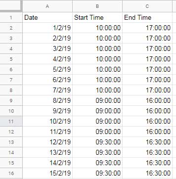
Screenshot # 1: Start and End Time in Time Format + Date Column.

Screenshot # 2: Start and End Time in Timestamp Format (No Date Column).

How to Calculate Hours Worked Per Week in Google Sheets

To create a summary report, no doubt, the Query is the ultimate solution. Of course, the Pivot Table built-in feature is there. But I am talking about the formula based solution.

You May Like: Drill Down Detail in Pivot Table in Google Sheets [Date Grouping].

When you try to calculate hours worked in week wise in Google Sheets, that using the function Query, you might face a few issues. What are they?

1. The first issue is, how to aggregate a time duration column in Query. This is because the Query doesn’t consider the time duration column as a number column. So obviously we can’t use it in calculations.
2. The second issue is related to the above, i.e., how to subtract end time from start time in Query using a simple arithmetic operator.

I am going to address these issues in my examples below. There is a workaround and in that, I have included every piece of information. So follow it carefully.

Further, here is my example Sheet to check the formula in live action.

From Work Start, End Time and Date Calculate Hours Worked in Week Wise in Google Sheets

First, refer to screenshot # 1 above. In that column A contains the date of work, B contains the start time of work, and C contains the end time of work.

Now, based on that data, see how to write a formula that can calculate hours worked in week wise in Google Sheets.

Step # 1:

In Week Wise summary, the first step is to extract the week number from the date column. Here is a suitable formula for that.

=ArrayFormula(if(Len(A2:A),Weeknum(A2:A),))

Note: Please check my Google Sheets Functions Guide to refer to any functions mentioned in this post.

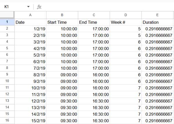
This would return the week numbers as below (in this week start day is considered as Sunday and the end day is obviously Saturday).

Note: Similar to the Weekday function, you can control the week start and end days in Weeknum function also.

For more info regarding this, please check my tutorial on Google Sheets Date Functions.

Step # 2:

In any blank column, in the first cell, just try this Query formula.

=query(B2:C,"Select C-B")

It would definitely return an error! Do you know the reason?

The reason is the contents in Column C and B are not numbers. So the function ‘difference’ (subtract) may not work in Query!

If you want to further test this, select the values in Column C and B and format it to numbers (Format > Numbers > Number). You can see that the Query works now!

Just undo the formatting. You can use the time functions hour, minute and second to solve this dilemma. How?

Must Check: The ultimate guide to Google Sheets Time functions.

Here is that awesome time to numerical value formula and the output just follows. Go through it carefully and you can understand what I have done.

=ArrayFormula(if(len(B2:B),(hour(C2:C)/24+minute(C2:C)/1440+second(C2:C)/86400)-(hour(B2:B)/24+minute(B2:B)/1440+second(B2:B)/86400),))

Step # 3:

Now we have two formulas. One returns week numbers and the other the time duration as numeric values.

Combine both the formulas to form a two column (virtual) array.

=ArrayFormula(if(len(A2:A),{Weeknum(A2:A),(hour(C2:C)/24+minute(C2:C)/1440+second(C2:C)/86400)-(hour(B2:B)/24+minute(B2:B)/1440+second(B2:B)/86400)},))

Step # 4:

Now you can use the above two columns as data in Query and calculate hours worked per week in Google Sheets. Here is that final step.

=Query(ArrayFormula(if(len(A2:A),{Weeknum(A2:A),(hour(C2:C)/24+minute(C2:C)/1440+second(C2:C)/86400)-(hour(B2:B)/24+minute(B2:B)/1440+second(B2:B)/86400)},)),"Select Col1, Sum(Col2) where Col1 is not null group by Col1")

Do format the time values in the formula output column to “Duration”. The instruction is written on the image.

The next question is how can I use the above formula in a timestamp column (please refer to the screenshot # 2 on the top)

From Start and End Timestamp Columns, Calculate Hours Worked in Week Wise in Google Sheets

No doubt the start and end time columns can also be timestamp columns. But it doesn’t matter. There are not much changes in the formula to use.

Our new sample data is in G2:H. There is no date column as both the column contain the timestamps.

In the above example, there are four steps. In the first step, we have populated the week numbers from column A. Here in the same formula use column G instead. It’s a timestamp (date time) column. But that’s not an issue.

In step # 2 there, I have converted the time duration to numeric values. Here also you can use the same formula.

Here Column B to be replaced by Column G and C to be replaced by column H.

Then combine the formulas as per step # 3 and the final formula as per step # 4 is here.

=Query(ArrayFormula(if(len(G2:G),{Weeknum(G2:G),(hour(H2:H)/24+minute(H2:H)/1440+second(H2:H)/86400)-(hour(G2:G)/24+minute(G2:G)/1440+second(G2:G)/86400)},)),"Select Col1, Sum(Col2) where Col1 is not null group by Col1")

That’s all. This way you can calculate hours worked in week wise in Google Sheets. Thanks for the stay, enjoy!

Additional Resources:

1. How to Create A Weekly Summary Report in Google Sheets.
2. How to Find Week Start Date and End Date in Google Sheets with Formula.
3. Weekday Name to Weekday Number in Google Sheets.
4. Query to Create Daily/Weekly/Monthly/Quarterly/Yearly Report Summary in Google Sheets.