This tutorial explains how to calculate hours worked per week in Google Sheets using the QUERY function and some simple helper formulas. Before you apply the QUERY, it’s important to structure your data correctly.

Follow along with the step-by-step instructions below. To try it yourself, you can copy the sample sheet.

Sample Data

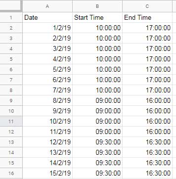
Assume you have a dataset with the following columns:

• Date (Column A)
• Start Time (Column B)
• End Time (Column C)

Using this data, you can easily calculate hours worked per week in Google Sheets.

You can also subtract a fixed lunch break (like 1 hour) if needed.

Step 1: Add a Week Number Column

In cell D1, enter the following formula:

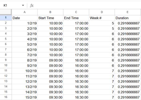
=VSTACK("Week #", ARRAYFORMULA(IF(LEN(A2:A), WEEKNUM(A2:A, 1), )))

This formula assigns a week number to each date in column A. By default, the week starts on Sunday. To start the week on Monday, change 1 to 2.

Step 2: Calculate Daily Work Duration in Decimal Format

In cell E1, use this formula:

=VSTACK("Duration", ARRAYFORMULA(IF(LEN(B2:B), C2:C - B2:B, )))

This subtracts the start time from the end time and returns the result in decimal (fraction of a day). For example, 0.2916667 represents 7 hours.

Optional: Subtract Fixed Lunch Break

To deduct 1 hour for lunch daily, use:

=VSTACK("Duration", ARRAYFORMULA(IF(LEN(B2:B), C2:C - B2:B - 1/24, )))

For a 30-minute break, replace 1/24 with 0.5/24.

Why Decimal Format?

QUERY requires numerical input, and decimal format is essential. Using VSTACK with a text header and IF ensures the result remains numeric. A plain formula like =ARRAYFORMULA(C2:C - B2:B) may display in time format and won’t work well inside QUERY.

Step 3: Calculate Hours Worked Per Week Using QUERY

Now that your data includes week numbers and durations, run the following QUERY:

=QUERY(D1:E, "SELECT Col1, SUM(Col2) WHERE Col1 IS NOT NULL GROUP BY Col1 FORMAT SUM(Col2) '[h]:mm:ss'", 1)

This will return the total hours worked for each week:

To learn how to rename columns in the result, check out How to Use the Label Clause in Google Sheets Query.

Step 4: Calculate Without Helper Columns (Optional)

If you prefer not to use extra columns, combine the logic using HSTACK and VSTACK:

=ARRAYFORMULA(HSTACK(
   VSTACK("Week #", IF(LEN(A2:A), WEEKNUM(A2:A, 1), )),
   VSTACK("Duration", IF(LEN(B2:B), C2:C - B2:B, ))
))

This creates a dynamic dataset you can plug directly into the QUERY function.

Conclusion

You now know how to calculate hours worked per week in Google Sheets—whether using helper columns or a single combined formula. With small adjustments, you can also deduct breaks or group hours by different date ranges.

Resources

• Creating a Weekly Summary Report in Google Sheets
• Finding Week Start and End Dates in Google Sheets: Formulas
• Summarize Data by Week Start and End Dates in Google Sheets
• Filter Data for a Specific Number of Past Weeks in Google Sheets
• How to Sum Values by the Current Week in Google Sheets