Using the QUERY function, you can convert text cases in specific columns of a table in Google Sheets to upper or lower case.
The QUERY function includes two scalar functions named UPPER and LOWER that are used for this purpose.
These scalar functions also play a key role in case-insensitive string matching within the QUERY function. When applying criteria to a column for case-insensitive filtering, you can specify the criteria in either lower case or upper case letters, and the values in the column will be converted accordingly for matching.
Let’s explore how to apply bulk text case conversion using the QUERY function in Google Sheets.
Bulk Text Case Change in Google Sheets Using QUERY Function
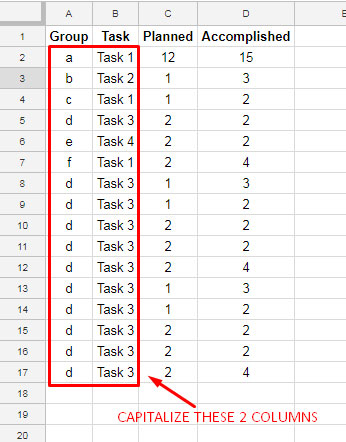
In the following sample data, I have data in columns A to D where columns A and B are text types. The data range is A1:D17, and the first row contains headers.
Sample Data:

Here are a few examples of using the QUERY function to bulk convert text cases in the first two columns:
Example 1:
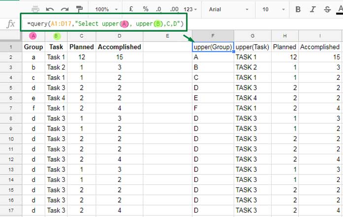
=QUERY(A1:D17, "SELECT UPPER(A), UPPER(B), C, D", 1)This formula changes the text case of values in columns A and B to uppercase letters.

It follows the syntax QUERY(data, query, [headers]) where:
data:A1:D17query:"SELECT UPPER(A), UPPER(B), C, D"headers:1(the number of header rows in the table. If omitted, the function will detect the number of header rows automatically)
Example 2:
If you want to convert one column to uppercase and another column to lowercase, use this formula:
=QUERY(A1:D17, "SELECT LOWER(A), UPPER(B), C, D", 1)Bulk Text Case Change Using QUERY While Retaining the Original Field Labels
An issue with applying bulk text changes using QUERY is the modification of headers (field labels).
When using scalar functions, you might encounter labels like upper(Group), upper(Task) if the headers are Group and Task, or upper(), upper() if there are no headers in the table.
To retain the original labels, you should use the LABEL clause:
=QUERY(A1:D17, "SELECT LOWER(A), UPPER(B), C, D LABEL LOWER(A) 'Group', UPPER(B) 'Task' ", 1)If your original table has no header row, you can remove the labels added by these scalar functions:
=QUERY(A1:D17, "SELECT LOWER(A), UPPER(B), C, D LABEL LOWER(A) '', UPPER(B) '' ", 1)Additional Note
We can’t apply the PROPER case in QUERY as there is no such scalar function available.


Dear Prashanth
I am not able to understand why you need to do it with a query. I think it can be done simply by an array function in one of the columns and then copy-paste-value only.
Am I missing something?
I was just introducing how to use LOWER/UPPER functions in Query.
The real purpose or real-life use of these two functions are not the bulk change case. It’s related to the case sensitivity of the Query function. I’ll write a tutorial on that and post the link below soon.
In the meantime, you can check the below tutorial to get some idea about the case sensitivity of the Query and what I am going to write about.
How to Use the Proper Function in Google Sheets Query.
Great work, very useful.
What is the regexp for taking out middle initials?
For example in; John,P. Steward
I want to take out every, initial. from every record in a column.
Any examples?
Thanks
Hi, Kenny,
Assume all the names in the column follows the same format. If so for a range B2:B, you can use the below REGEX in C2.
=ArrayFormula(IF(LEN(B2:B),REGEXEXTRACT(B2:B, "\,([A-Za-z]+)\."),))This formula would extract the initials separated by a command and a full stop as the separators.
Best,