If you’re tired of forgetting what you’ve read, which books you rated 5 stars, or how many unread titles are in your backlog — it’s time to build an advanced book tracker in Google Sheets.

In this tutorial, I’ll walk you through creating a fully customizable and advanced reading list spreadsheet — complete with dropdowns for status and genre, star ratings, summary metrics, and a dashboard with charts that visualize your reading habits.

Whether you’re organizing your TBR list or analyzing your reading stats, this tracker has you covered — and the best part is, you don’t need any add-ons or fancy tools. Just Google Sheets.

Let’s see how to build a book tracker template in Google Sheets step-by-step.

✨ Want a ready-made version with extra charts and polished formatting?
Check out the Google Sheets Reading List Tracker Template (Free Download) — it’s a more advanced version of the tracker we’ll build in this tutorial.

Step 1: Set Up Your Book Tracker in Google Sheets

1. Go to sheets.new to open a new spreadsheet.
2. Click the + button at the bottom-left corner twice to add two more sheets.
3. Rename:
   • First sheet → Data
   • Second sheet → Dashboard
   • Third sheet → Calculations
4. Rename the file from “Untitled spreadsheet” to something like Advanced Book Tracker.

Step 2: Data Entry Sheet Setup

On the Data sheet, enter the following headers in row 2 (columns A to J):

Title | Author | Country | Genre | Source | Status | Rating | Start Date | Finish Date | Notes

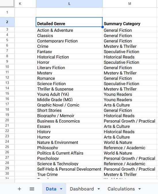
1. Convert to Table: Select A2:J3, right-click → Convert to table.
2. In columns L and M, paste your genre mapping table:
   • Column L: Sub-Genres
   • Column M: Main Genre Categories
     (e.g., Mystery → Mystery & Thriller)

Add Dropdowns

• Genre (D3) → Insert > Dropdown > From range → L3:L
• Source (E3) → Dropdown → Enter Owned, Borrowed
• Status (F3) → Dropdown → Completed, TBR, Reading, DNF
• Rating (G3) → Insert > Smart Chips > Rating
• Start/Finish Dates (H3/I3) → Format > Number > Date
• Wrap Headers → Select A2:J3 → Format > Wrapping > Wrap

Note: If you aren’t familiar with drop-downs, check out this guide: The Best Data Validation Examples in Google Sheets

Add Mock Data (Example):

Step 3: Core Formulas in the Calculations Sheet

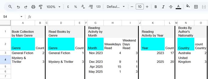
a. Book Collection by Main Genre

In cell A1, enter:

Book Collection by Main Genre

In cell A2, paste this formula:

=ArrayFormula(
   QUERY(
      XLOOKUP(Table1[Genre], Data!L3:L, Data!M3:M), 
      "select Col1, Count(Col1) where Col1 is not null group by Col1 label Col1 'Genre', count(Col1) 'Count'", 0
   )
)

What it does:

• XLOOKUP(...): Maps the sub-genres (from your Genre column) to their respective main genres.
• QUERY(...): Groups the main genres and counts how many books fall into each.

b. Read Books by Genre

In cell D1, enter:

Read Books by Genre

In cell D2, enter:

=ArrayFormula(
   QUERY(
      HSTACK(
         XLOOKUP(Table1[Genre], Data!L3:L, Data!M3:M), Table1[Status]
      ), 
      "select Col1, Count(Col1) where Col2='Completed' group by Col1 label Col1 'Genre', count(Col1) 'Count'", 0
   )
)

What it does:

• XLOOKUP(...): Returns the main genre corresponding to each sub-genre.
• HSTACK(...): Joins the main genre and status columns side by side.
• QUERY(...): Filters for rows with “Completed” status, groups by genre, and counts.

c. Reading Activity by Month (Weekdays vs. Weekends)

In G1, type:

Reading Activity by Month

In G2, paste this advanced formula:

=QUERY(
   IFERROR(WRAPROWS(TOROW(
      LET(
         table, FILTER(HSTACK(Table1[Start Date], Table1[Finish Date]), Table1[Status]="Completed"), 
         MAP(CHOOSECOLS(table, 1), CHOOSECOLS(table, 2), LAMBDA(_start, _end, TOROW(
            ARRAYFORMULA(LET(
               start, INT(_start), 
               end, INT(_end), 
               full_months, EDATE(EOMONTH(start, -1)+1, SEQUENCE(DATEDIF(start, end, "M"))), 
               boundary_dates_list, UNIQUE(TOCOL(VSTACK(start, full_months, IF(EOMONTH(start, 0)=EOMONTH(end, 0),, EOMONTH(end, -1)+1), end), 3)),
               data, HSTACK(EOMONTH(boundary_dates_list, -1)+1, CHOOSEROWS(boundary_dates_list, SEQUENCE(ROWS(boundary_dates_list)-1, 1, 2))-boundary_dates_list-VSTACK(1, SEQUENCE(ROWS(boundary_dates_list)-1, 1, 0, 0)), VSTACK(1, TOCOL(SEQUENCE(ROWS(boundary_dates_list)-2, 1, 0, 0), 3), 1)), 
               data
            ))
         )))
      )), 3)
   ), "select Col1, sum(Col2), sum(Col3) where Col1 is not null group by Col1 label Col1 'Month', sum(Col2) 'Weeekdays Read', sum(Col3) 'Weekend Days Read' format Col1 'MMM YYYY'", 0
)

What it does:

• Splits your reading period into days by month.
• Calculates how many were weekdays and how many were weekends.
• Summarizes that by month.

💡 Note: This is an advanced formula. For a complete breakdown, check out: Calculate Trip Days by Month (Start, End, and Full Days) in Google Sheets

d. Reading Activity by Year

In K1, type:

Reading Activity by Year

In K2, enter:

=IFERROR(
   QUERY(
      G2:I, 
      "select year(Col1), sum(Col2)+sum(Col3) where Col1 is not null group by year(Col1) label year(Col1) 'Year', sum(Col2)+sum(Col3) 'Count' ", 1
   )
)

What it does:

• Extracts the year from each month.
• Sums up weekday and weekend reading days per year.

e. Books by Author’s Nationality

In N1, type:

Books by Author's Nationality

In N2, enter:

=QUERY(
   Table1[[#ALL],[Country]], 
   "select Col1, count(Col1) where Col1 is not null group by Col1", 1
)

What it does:

• Groups books by country listed in the Author column.
• Returns the number of books per nationality.

Step 4: Build the Dashboard

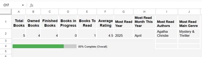
Enter these summary labels in Dashboard A1:J1:

Total Books | Owned Books | Finished Books | Books in Progress | Books To Read | Avg Rating | Most Read Year | Most Read Month | Top Authors | Top Genre

Below each cell, enter the following formulas to calculate your reading stats:

=COUNTA(Table1[Title])

Returns the total number of books you’ve listed (both owned and borrowed).

=COUNTIFS(Table1[Source], "Owned")

Counts how many of those books are owned.

=COUNTIF(Table1[Status], "Completed")

Returns the number of books you’ve finished reading.

=COUNTIF(Table1[Status], "Reading")

Counts books that are currently in progress.

=COUNTIF(Table1[Status], "TBR")

Counts books marked as “To Be Read.”

=IFERROR(
   AVERAGEIF(Table1[Status], "Completed", Table1[Rating])
)

Calculates your average rating for completed books (ignores errors if there are no ratings yet).

=TEXTJOIN(" | ", TRUE, 
   FILTER(Calculations!K3:K, Calculations!L3:L=MAX(Calculations!L3:L))
)

Displays your most read year(s), using a pipe “|” if there’s a tie.

=LET(
   cYear, FILTER(Calculations!G3:I, YEAR(Calculations!G3:G)=YEAR(TODAY())), 
   top, SORTN(cYear, 1, 0, CHOOSECOLS(cYear, 2)+CHOOSECOLS(cYear, 3), false), 
   IFERROR(
      TEXT(CHOOSECOLS(top, 1), "MMMM")
   )
)

Shows your most read month in the current year based on completed page count.

=ARRAY_CONSTRAIN(
   SORTN(
      QUERY(
         HSTACK(Table1[Author], Table1[Status]), 
         "select Col1, count(Col1) where Col2='Completed' group by Col1 label count(Col1)''", 0
      ), 1, 1, 2, FALSE
   ), 3, 1
)

Returns your most read author — up to three authors if there’s a tie.

=ARRAY_CONSTRAIN(
   SORTN(Calculations!D3:E, 1, 1, 2, FALSE
   ), 3, 1
)

Returns your most read main genre — up to three genres if there’s a tie.

Reading Progress Bar

A4:

=SPARKLINE({C2, A2}, {"charttype", "bar"; "Color1", "#4CAF50"; "Color2", "#cccccc"; "min", 0; "max", A2})

This formula creates a bar-style sparkline (a mini in-cell chart) that visually shows progress toward a goal.

E4:

=IFERROR(JOIN(" ",to_percent(C2/A2), "Complete (Overall)"))

This formula calculates the overall completion percentage and displays it as a formatted text string like:
75% Complete (Overall)

Step 5: Add Charts to the Dashboard

We’ll create four charts to visualize your reading data: two pie charts, one stacked bar chart, and one Geo chart. All the chart data lives in the Calculations sheet. You’ll insert the charts there first, and then move them to the Dashboard.

Book Collection by Genre (Pie Chart)

1. Go to the Calculations sheet.
2. Select the range A2:B.
3. Click Insert > Chart.
4. In the Chart Editor, change the chart type to Pie chart (if it’s not already).
5. Switch to the Customize tab, expand Chart & axis titles, and set the chart title to:
   “Book Collection by Genre”
6. Click the chart > Edit menu > Copy.
7. Switch to the Dashboard sheet and Paste the chart.
8. Drag to position it and resize by adjusting the edges.
9. Go back to Calculations and delete the chart to keep the sheet tidy.

Read Books by Genre (Pie Chart)

1. Select the range D2:E in the Calculations sheet.
2. Insert a Pie Chart and title it:
   “Read Books by Genre”
3. Copy and paste the chart into the Dashboard.
4. Resize and position it as needed, then delete the original from Calculations.

Reading Activity by Month (Stacked Bar Chart)

1. Select the range G2:I in the Calculations sheet.
2. Insert a chart, and in the Chart Editor, choose Stacked Bar Chart.
3. Under the Customize tab > Chart & axis titles, set the title to:
   “Reading Activity by Month”
4. Copy and paste it into the Dashboard and delete the original.

Books by Country (Geo Chart)

1. Select the range N3:O in the Calculations sheet.
2. Insert a chart and change the chart type to Geo Chart.
3. Copy and paste it into the Dashboard, then remove the original from Calculations.

Related

If you followed the steps above, you’ve now created your own advanced book tracker — complete with dropdowns, summaries, and a visual dashboard.

👉 You can make a copy of the same sample sheet built in this tutorial here: Sample Tracker Sheet

🔥 Want an even more polished version with bonus charts, formatting tweaks, and enhancements?
Check out the Google Sheets Reading List Tracker Template (Free Download).