The RANK function in Google Sheets is commonly used to assign rankings to numerical data. However, when multiple values are identical, the function assigns them the same rank, creating ties. Since RANK only considers numbers, it does not differentiate tied values based on other criteria, such as alphabetical order. This tutorial will show you how to break RANK ties alphabetically in Google Sheets using a formula.
An added advantage of this formula is that it doesn’t require any helper range and automatically expands to accommodate new data.
Formula to Break RANK Ties Alphabetically
You can use the following formula to break RANK ties alphabetically in Google Sheets:
=ArrayFormula(IFERROR(LET(data, SORT(HSTACK(ROW(points), names, points), 2, 1), col, CHOOSECOLS(data, 3), rnk, RANK(col, col, FALSE), cnt, COUNTIFS(col, col, ROW(points), "<="&ROW(points))-1, SORT(rnk+cnt, CHOOSECOLS(data, 1), 1))))Explanation of Parameters:
points– The numeric column containing the values to be ranked.names– The text column used to break ties alphabetically.
By default, the formula assigns rank 1 to the highest value in points. If you want to rank the lowest value as 1, replace FALSE with TRUE in the RANK function.
Understanding the RANK Tie Issue
When using the RANK function to rank numerical data, identical values receive the same rank. However, the next rank is skipped, causing gaps in the ranking sequence.
For example:
| Player Names | Points | Rank |
| Tony | 12 | 1 |
| Alex | 5 | 5 |
| Myrtle | 11 | 2 |
| Ellen | 11 | 2 |
| Javier | 7 | 4 |
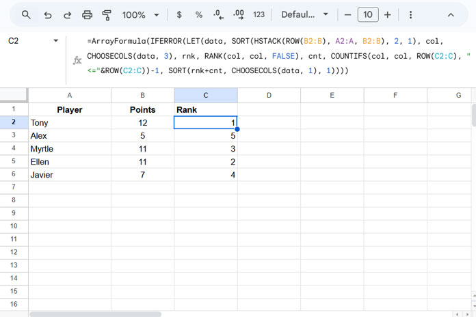
Here, Myrtle and Ellen both have 11 points, so they are assigned the same rank (2). If we want to differentiate them further, we can break the tie alphabetically.
Example: Breaking RANK Ties Alphabetically
Assume the above dataset is in A2:B. To return ranks without ties, use the following formula in C2:
=ArrayFormula(IFERROR(LET(data, SORT(HSTACK(ROW(B2:B), A2:A, B2:B), 2, 1), col, CHOOSECOLS(data, 3), rnk, RANK(col, col, FALSE), cnt, COUNTIFS(col, col, ROW(B2:B), "<="&ROW(B2:B))-1, SORT(rnk+cnt, CHOOSECOLS(data, 1), 1))))This formula breaks RANK ties alphabetically based on player names.

Key Points:
- This is an array formula, so there’s no need to drag it down manually.
- It will automatically calculate rankings for the entire dataset.
Formula Logic and Explanation
Logic:
The formula first sorts the data alphabetically by name and then calculates rankings. By subtracting 1 from the running count of points, adding it to the rank, and finally sorting the ranks based on row numbers, it ensures that ties are broken alphabetically.
Step-by-Step Breakdown:
- Sort Data by Name:
SORT(HSTACK(ROW(B2:B), A2:A, B2:B), 2, 1)- Creates an array with row numbers, player names, and points.
- Sorts this array by player name in ascending order.
- Extract the Points Column:
CHOOSECOLS(data, 3)- Selects the points column from the sorted data.
- Rank the Points Column:
RANK(col, col, FALSE)- Ranks the values in the points column.
- Calculate Running Count:
COUNTIFS(col, col, ROW(C2:C), "<="&ROW(C2:C))-1- Counts the occurrences of each score up to the current row and subtracts 1 to adjust the ranking.
- Adjust and Sort the Final Ranks:
SORT(rnk+cnt, CHOOSECOLS(data, 1), 1)- Adds the rank and running count, ensuring unique rankings.
- Sorts results back into the original row order.
Conclusion
Using this method, you can break RANK ties alphabetically in Google Sheets, ensuring a clear and logical ranking system. Whether you’re sorting competition scores, student grades, or sales figures, this technique helps maintain a structured ranking without duplicate ranks.


