


")


")


When using the GROUP BY clause in the QUERY function in Google Sheets, the result is automatically sorted by the group column. While this behavior works well in most cases, it can be limiting if you want to retain the original data order.
If you’re looking to fix the auto-sorting issue in QUERY GROUP BY in Google Sheets, there’s no built-in setting to turn it off. However, you can use a clever formula workaround with LET, XMATCH, and SORT to restore the original row order.
Let’s dive in.
The Problem: QUERY GROUP BY Auto-Sorts the Output
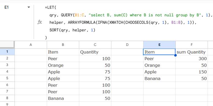
Here’s a sample dataset in range B1:C:
| Item | Quantity |
| Peer | 100 |
| Orange | 50 |
| Apple | 75 |
| Apple | 75 |
| Peer | 100 |
| Peer | 100 |
| Banana | 50 |
Now try this standard QUERY formula:
=QUERY(B1:C, "select B, sum(C) where B is not null group by B", 1)Result:
| Item | sum Quantity |
| Apple | 150 |
| Banana | 50 |
| Orange | 50 |
| Peer | 300 |
Notice how the fruits are automatically sorted alphabetically? That’s the default behavior of GROUP BY.
Expected Result: Maintain Original Group Order
What if you want the output in the order that fruits first appear in the source data?
| Item | sum Quantity |
| Peer | 300 |
| Orange | 50 |
| Apple | 150 |
| Banana | 50 |
Here’s how you can achieve that.
Fix Auto-Sorting Issue in QUERY GROUP BY: The Formula
Use the following formula to preserve the original order of the grouped values:
=LET(
   qry, QUERY(B1:C, "select B, sum(C) where B is not null group by B", 1),
   helper, ARRAYFORMULA(IFNA(XMATCH(CHOOSECOLS(qry, 1), B1:B), 1)),
   SORT(qry, helper, 1)
)
How the Formula Works
Let’s break it down:
LET(): Assigns names to parts of the formula to make it cleaner and more efficient.qry:QUERY(B1:C, "select B, sum(C) where B is not null group by B", 1)
This is your standard query. It groups by the “Items” column and sums the quantities.helper:ARRAYFORMULA(IFNA(XMATCH(CHOOSECOLS(qry, 1), B1:B), 1))CHOOSECOLS(qry, 1)
pulls just the group names from the query result.XMATCH(..., B1:B)
finds the first appearance of each group name in the original data.IFNA(..., 1)
ensures the header row returns 1 (instead of an error).
SORT(qry, helper, 1):
Reorders the query output using the helper column—restoring the original data order.
Does This Work with a PIVOT Clause?
Yes, this method works with pivot queries too.
Here’s a dataset with an added “Category” column in range A1:C:
| Category | Items | Quantity |
| Imported | Peer | 100 |
| Local | Orange | 50 |
| Local | Apple | 75 |
| Imported | Apple | 75 |
| Imported | Peer | 100 |
| Local | Peer | 100 |
| Imported | Banana | 50 |
Use this formula:
=LET(
   qry, QUERY(A1:C, "select B, sum(C) where B is not null group by B pivot A", 1),
   helper, ARRAYFORMULA(IFNA(XMATCH(CHOOSECOLS(qry, 1), B1:B), 1)),
   SORT(qry, helper, 1)
)
It works the same way—preserving the order of the “Fruits” column as they first appear in the source, even with pivoted columns.
Conclusion
The QUERY function in Google Sheets automatically sorts grouped results—often helpful, but sometimes frustrating. Thankfully, using LET, XMATCH, and SORT, you can easily fix the auto-sorting issue in QUERY GROUP BY and maintain your original data order.
This approach is clean, flexible, and works even with pivot clauses—making it ideal for custom reports or dashboards.