Average Top N Percent Values in Google Sheets (With or Without Conditions)

To calculate the average of the top N percent of values in Google Sheets, you can use the PERCENTILE function as a threshold within AVERAGEIF.

If you’d like to calculate the average of the top N percent of values based on a condition, simply use PERCENTILE with AVERAGEIFS.

Even better? You can replace AVERAGEIF and AVERAGEIFS with a more flexible combination using AVERAGE + FILTER. Let’s explore all these approaches below.

How to Calculate the Average of Top N Percent Values Without a Condition

Let’s start with a basic example.

Goal: Find the average of the top 20% of values in a dataset.

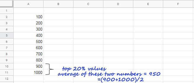
Chart showing the average of the top N percent of values without any condition in Google Sheets

We’ll use the PERCENTILE function to get the cutoff point, then apply it within either FILTER or AVERAGEIF to isolate the top 20%.

Step 1: Find the PERCENTILE Value

=PERCENTILE(A2:A11, 80%)

This returns the value at the 80th percentile, since the top 20% of values lie above the 80th percentile (100% – 20%).

Step 2: Filter Top 20% of Values

To see only the top 20% values:

=FILTER(A2:A11, A2:A11 > PERCENTILE(A2:A11, 80%))

Step 3: Average the Top 20% Values

Wrap the above in AVERAGE:

=AVERAGE(FILTER(A2:A11, A2:A11 > PERCENTILE(A2:A11, 80%)))

Alternatively, you can use AVERAGEIF without needing to filter:

=AVERAGEIF(A2:A11, ">" & PERCENTILE(A2:A11, 80%))

Both formulas will give you the average of the top 20% values.

How to Calculate the Average of Top N Percent Values With a Condition

Now let’s add a condition to the calculation.

Scenario: Calculate the average of the top 20% of sales values only for the “South” region.

Table showing the average of the top 20% values based on a condition in Google Sheets

Sample Data Layout:

Column C: Region
Column D: Sales

Option 1: AVERAGEIFS with Condition

=AVERAGEIFS(D2:D, C2:C, "South", D2:D, ">" & PERCENTILE(D2:D, 80%))

This formula averages only the sales values greater than the 80th percentile and from the “South” region.

Option 2: AVERAGE + FILTER with Condition

=AVERAGE(FILTER(D2:D, C2:C = "South", D2:D > PERCENTILE(D2:D, 80%)))

This version works similarly but offers more flexibility in case you need to stack multiple conditions.

Summary

To calculate the average of the top N percent of values in Google Sheets:

Use PERCENTILE to determine the threshold.
Combine it with AVERAGEIF or AVERAGEIFS for a compact solution.
Use AVERAGE + FILTER for more control and readability.

Whether or not you have conditions, both methods work effectively.