Auto-Fill Sequential Dates When Value Entered in Next Column in Google Sheets

Published on

To auto-fill sequential dates in Google Sheets, we can depend on a very simple formula or the fill handle in Google Sheets.

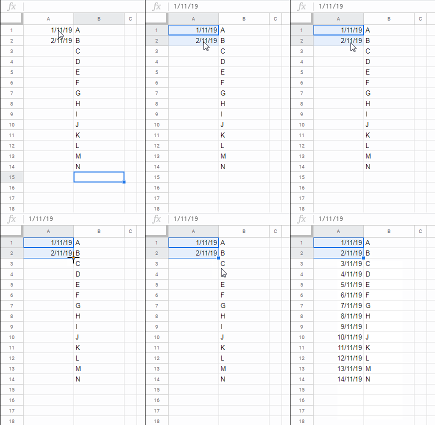
The fill handle works like this. You enter a date in one cell and another date in an adjoining cell.

For example, enter the date 01 Nov 2019 in cell A1 and 02 Nov 2019 in cell A2. To auto-fill sequential dates, select these two cells and double click on the fill handle.

Sequential dates using fill handle

This will fill dates up to the last row containing a value in the next column.

This manual auto-filling of sequential dates in Google Sheets has one problem. If you enter more values in column B, again you need to repeat the same.

As an example, I have entered values in cells B15, B16, and B17. To extend the sequential dates up to row # 17, I must select the dates in cell A13 and A14 and double click the fill handle again.

We can automate the same using a formula. I mean we can write a formula in cell A1 to auto-fill sequential dates up to the last non-blank row in the adjoining column.

Array Formula to Auto-Fill Sequential Dates Based on Next Column in Google Sheets

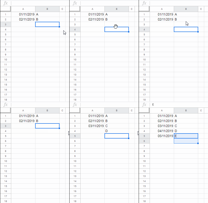
First of all, let me show you what I am talking about.

Auto-fill sequential dates in Google Sheets using a formula

Quite interesting, right?

Here is the array formula that I have used in cell A1 in the example above (see the GIF).

=sequence(counta(B1:B),1,date(2019,11,1))

This formula may return numbers (date values) instead of proper dates. So before entering the formula, select column A and format it to dates.

Read: How to Utilise Google Sheets Date Functions [Complete Guide].

The date formatting is under the menu Format > Number > Date.

How Does This Formula Work?

Dates in Google Sheets or any other spreadsheets are actually recorded as numbers. To find the underlying number of dates, you can use the DATEVALUE function. For example, see the below formula.

=DATEVALUE(today())

That means we can use the dates in the Sequence function to return a grid of sequential dates.

Syntax:

SEQUENCE(rows, [columns], [start], [step])

From this syntax, you can understand one thing without my explanation and that is the ‘start’ argument. That is to replace the ‘start’ with the start date in the sequence.

In my formula, it’s 01 Nov 2019 which to be used as date(2019,11,1). So you won’t face any issue related to regional date settings like mm/dd/yyyy or dd/mm/yyyy.

We want to auto-fill the sequential dates in only one column. So use 1 as the ‘columns’. The arguments left are ‘rows’ and ‘step’.

We can find the number of rows to be filled by sequential dates using the ‘rows’ argument. I have used counta(B1:B) which counts the values in column B.

Read: How to Use All Google Sheets Count Functions [All 8 Count Functions].

If there are 3 rows filled with values in column B, the Sequential formula will return sequential dates in three rows. This is because the COUNTA will feed ‘rows’ with the number 3.

The ‘step’ value is not useful for sequential dates or numbers. To understand this argument, modify my formula as below to include ‘step’ value 2.

=sequence(counta(B1:B),1,date(2019,11,1),2)

The result will be alternate dates like 01 Nov 19, 03 Nov 19, 05 Nov 19 and so on.

Auto-Fill Sequential Dates Excluding Hidden/Filtered Out Rows in Google Sheets

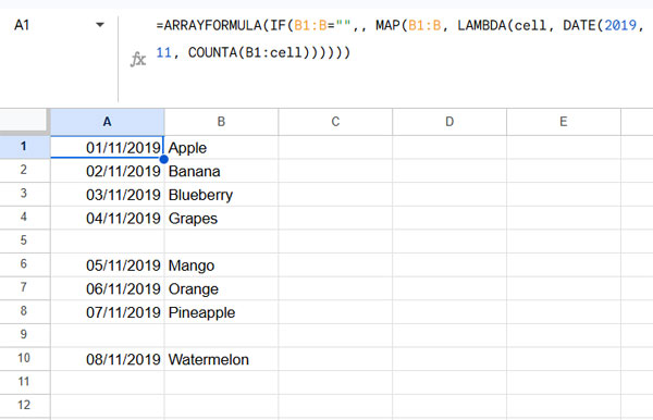
If you want you can autofill sequential dates only in the visible rows.

Things to Know Before We Start

In Google Sheets, to exclude hidden rows (or rows that are filtered out) in formulas, as far as I know, we may require a helper column.

Of course, you can overcome this limitation in a limited way with a virtual helper column which I have experimented in one of my earlier tutorials here – Google Sheets Query Hidden Row Handling with Virtual Helper Column.

It will work only in a limited data range. So I am going with a helper column instead of a virtual helper column here.

Here in our example, column C is the helper column. Enter this COUNTA equivalent in cell C1 and copy-paste up to the last row in that column. We can definitely hide this column at any point of time.

Subtotal Function as Counta Using 103
=subtotal(103,B1)

Related: Subtotal Function With Conditions in Excel and Google Sheets.

The 103 function number in Subtotal works as COUNTA equivalent. But this function has one advantage over the COUNTA. What’s that?

The Subtotal Counta will return 0 if the row that contains this formula keyed in is hidden/filtered out.

For example, if you hide the row # 3, the value (count) in cell C3 will be 0.

Steps Involved

In our first example, the Sequence formula is keyed in cell A1. Cut that formula and paste it in cell F1.

Then replace the COUNTA in that Sequence formula with the following COUNTIF.

countif(C1:C,">0")

Why so?

Note: To learn Docs Sheets functions, please refer to my Google Sheets Functions Guide.

It’s because the Counta returns the count of total non-blank rows based on values in column B whereas the Countif returns the count of total non-blank rows excluding hidden rows based on values in column B.

So the formula in cell F1 to auto-fill dates in visible rows will be as follows.

=sequence(countif(C1:C,">0"),1,date(2019,11,1),2)

This formula won’t work as expected. We should make some more changes.

In cell E1, enter the below formula to return the row numbers excluding hidden rows. I am skipping explaining this formula as it may confuse you. Simply use it.

=filter(row(indirect("A1:A"&counta(B1:B))),indirect("C1:C"&counta(B1:B))>0)

Now my example sheet will look like as follows.

Row numbers of visible rows in Google Sheets

In cell A1, I will write a Vlookup formula that will use the above E1:F as the range.

Syntax:

VLOOKUP(search_key, range, index, [is_sorted])

The search_key(s) will be row numbers and the index will be the second column in the range that is the values in column F.

=ArrayFormula(IFNA(vlookup(Row(A1:A),E1:F,2,0)))

We can replace E1:F with the corresponding two formulas in E1 and F1 as below.

={filter(row(indirect("A1:A"&counta(B1:B))),indirect("C1:C"&counta(B1:B))>0),sequence(countif(C1:C,">0"),1,date(2019,11,1))}

The final Vlookup formula in cell A1 with the above formula as the range.

=ArrayFormula(IFNA(vlookup(Row(A1:A),{filter(row(indirect("A1:A"&counta(B1:B))),indirect("C1:C"&counta(B1:B))>0),sequence(countif(C1:C,">0"),1,date(2019,11,1))},2,0)))

We are now ready to test the formula. Hide any row and see the date adjusts accordingly.

Auto-fill sequential dates excluding hidden rows in Google Sheets

You have learned two tips in this tutorial.

  1. Autofill sequential dates when values are entered in the next column.
  2. Sequential dates excluding hidden/filtered out rows plus point # 1 above.

Thanks for the stay. Enjoy!

Prashanth KV
Prashanth KV
Your Trusted Google Sheets and Excel Guide Prashanth KV brings a wealth of experience in Google Sheets and Excel, cultivated through years of work with multinational corporations in Mumbai and Dubai. As a recognized Google Product Expert in Docs Editors, Prashanth shares his expertise through insightful blogging since 2012. Explore his blog for practical tips and guidance on maximizing your spreadsheet skills.

Highlight Upcoming Birthdays in Google Sheets

When highlighting upcoming birthdays in Google Sheets, one important aspect is ignoring the year...

Compare Two Tables for Differences in Excel

To compare two tables with similar data for differences, you can use the XLOOKUP...

Calculate Weighted Average in Pivot Table in Google Sheets

You can calculate a weighted average in a Pivot Table using a custom formula...

Summarize Data and Keep the Last Record in Google Sheets

In Google Sheets, we can summarize data (like sum, average, min, max, count) using...

More like this

Highlight Upcoming Birthdays in Google Sheets

When highlighting upcoming birthdays in Google Sheets, one important aspect is ignoring the year...

Calculate Weighted Average in Pivot Table in Google Sheets

You can calculate a weighted average in a Pivot Table using a custom formula...

Summarize Data and Keep the Last Record in Google Sheets

In Google Sheets, we can summarize data (like sum, average, min, max, count) using...

LEAVE A REPLY

Please enter your comment!
Please enter your name here

This site uses Akismet to reduce spam. Learn how your comment data is processed.