


")


")

")
")
 in Excel & Google Sheets")


If you manage customer invoices in Google Sheets, you’ll eventually need to allocate payment receipts—whether they match invoices exactly, are partial installments, or come as lump-sum amounts. This tutorial shows you how to handle all these scenarios using formulas like VLOOKUP, QUERY, SUMIF, and MIN.
When Is Payment Allocation Needed?
Let’s consider a few practical scenarios:
- One-to-one match: You receive a full payment for a specific invoice.
- Installments: A single invoice is paid through multiple smaller payments.
- Lump-sum payment: You receive one payment that covers multiple invoices but doesn’t reference invoice numbers.
This tutorial explains how to handle all of these situations using a Google Sheets-based allocation model.
Sample Invoice Data for Allocation
Start by copying this sample account statement into a new Google Sheets file in the range Sheet1!A1:F12.
Table 1: Invoice Data
| Customer | Invoice Date | Invoice # | Debit | Credit | Balance |
|---|---|---|---|---|---|
| A | 23/06/19 | RA-8041 | 3578.80 | ||
| A | 23/06/19 | RA-8042 | 2967.92 | ||
| A | 23/06/19 | RA-8044 | 12742.84 | ||
| A | 23/06/19 | RA-8045 | 6801.52 | ||
| B | 14/07/19 | RA-8049 | 7995.00 | ||
| B | 20/08/19 | RA-8058 | 63892.80 | ||
| C | 21/08/19 | RA-8104 | 52248.00 | ||
| C | 21/08/19 | RA-8110 | 79803.63 | ||
| C | 21/08/19 | RA-8119 | 40423.86 | ||
| D | 01/09/19 | RA-8120 | 5000.00 | ||
| D | 01/09/19 | RA-8121 | 11000.00 |
Match One-Time Payments to Invoices Using VLOOKUP
Assume you’ve received payments like this (in Sheet2!A1:B4):
Table 2: Payment Receipts
| Invoice # | Receipt Amount |
|---|---|
| RA-8045 | 6801.52 |
| RA-8042 | 2967.92 |
| RA-8110 | 79803.63 |
To match these payments in Sheet1, enter the following formula in Sheet1!E2 (the Credit column):
=ArrayFormula(IFNA(VLOOKUP(C2:C, Sheet2!A2:B, 2, 0)))This is an array formula that automatically spills down the column and fills in the matched receipt amounts for all invoice numbers listed in Column C.
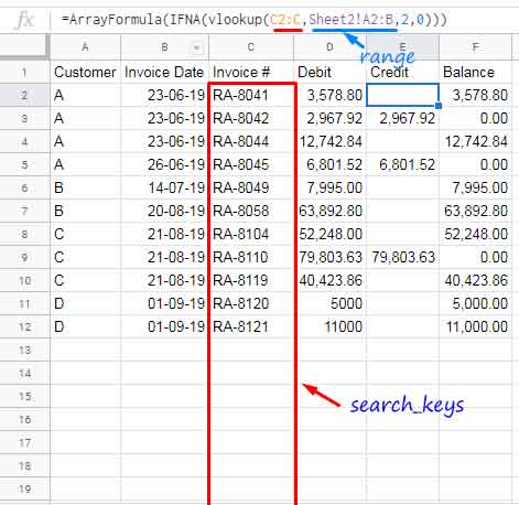
How It Works:
- VLOOKUP searches for invoice numbers from
Sheet1!C2:Cin Table 2. - If it finds a match, it returns the corresponding receipt amount.
- You can expand both Table 1 (invoices) and Table 2 (payments) with new entries. Thanks to the open-ended range (
C2:CandSheet2!A2:B), the ArrayFormula dynamically picks up any new data without needing to adjust the formula.
Allocate Partial Payments Using SUMIF
What if a customer pays in multiple installments against a single invoice?
For example, update Table 2 like this (range Sheet2!A1:B5):
| Invoice # | Receipt Amount |
|---|---|
| RA-8045 | 3400.76 |
| RA-8045 | 3400.76 |
| RA-8042 | 2967.92 |
| RA-8110 | 79803.63 |
In this case, using a basic VLOOKUP will only return the first match for RA-8045, ignoring subsequent payments. To correctly allocate partial payments, we need to summarize the total payment received per invoice.
Use SUMIF to Aggregate and Allocate
Enter the following formula in Sheet1!E2 (Credit column):
=ArrayFormula(IF(C2:C = "", , SUMIF(Sheet2!A2:A, C2:C, Sheet2!B2:B)))How It Works:
- SUMIF adds up all payment amounts in
Sheet2!B2:Bwhere the invoice number inSheet2!A2:Amatches the invoice inSheet1!C2:C. - The formula automatically handles repeated invoice numbers and returns the total amount received for each one.
- ArrayFormula ensures it spills down automatically, no need to drag.
This formula gives you an accurate match whether a payment was made in full or across multiple transactions. It’s especially useful for installment-based payments where the same invoice appears more than once.
Tip for advanced users: You can achieve the same result using a QUERY to group receipts, then look them up with VLOOKUP. While functional, this approach is more complex and offers no major advantage over SUMIF in this case.
=ArrayFormula(IFNA(VLOOKUP(C2:C, QUERY(Sheet2!A1:B, "SELECT A, SUM(B) WHERE A IS NOT NULL GROUP BY A", 1), 2, 0)))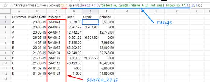
Allocate Payments Without Invoice Numbers (By Customer Name)
If you receive a payment without invoice references, but only the customer name, you can still allocate it.
Table 3: Payments Without Invoice Reference (in Sheet2!A1:B6):
| Customer | Receipt |
|---|---|
| A | 5000.00 |
| A | 6500.00 |
| B | 5000.00 |
| C | 10500.00 |
| D | 8000.00 |
Use this formula in Sheet1!E2 (Credit column) and drag it down manually:
=MIN(D2, SUMIF(Sheet2!$A$2:$A, A2, Sheet2!$B$2:$B) - SUMIF($A$1:A1, A2, $E$1:E1))Note:
This formula allocates payments only up to the total of invoiced amounts. If a customer pays more than the total due, any excess payment won’t be reflected in the allocation—it will remain untracked.
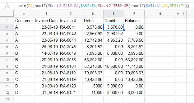
How This Formula Allocates Payments:
- First SUMIF: Gets the total receipts for that customer.
- Second SUMIF: Calculates how much has already been allocated to that customer so far (running total).
- MIN: Ensures you don’t allocate more than the invoice amount.
This method works for full, partial, or lump-sum payments per customer.
Optional: Customer-Wise Receipt Summary (Alternative Approach)
If you want to see the total receipts received per customer—regardless of how they are allocated—you can use one of the following formulas in a helper column (e.g., cell G2 in Sheet1).
Option 1: Using QUERY + VLOOKUP
=ArrayFormula(IFNA(VLOOKUP(A2:A, QUERY(Sheet2!A1:B, "SELECT A, SUM(B) WHERE A IS NOT NULL GROUP BY A", 1), 2, 0)))- This formula groups the receipts in
Sheet2by customer and returns the total amount received for each. VLOOKUPthen matches this total back to each row inSheet1based on the customer name.
Option 2: Using SUMIF as an Array Formula
=ArrayFormula(SUMIF(Sheet2!$A$2:$A, A2:A, Sheet2!$B$2:$B))- This formula also returns the total receipts per customer directly using SUMIF.
- It’s more concise and works just as well for this summary purpose.
These formulas are useful for reporting or cross-checking purposes—such as verifying how much each customer has paid in total. However, they do not allocate payments to specific invoices. For that, use the MIN + SUMIF allocation formula explained earlier.
Calculate Outstanding Balance
To find the remaining balance for each invoice, enter this formula in Sheet1!F2:
=ArrayFormula(IF(LEN(A2:A), D2:D - E2:E, ))This subtracts the allocated amount from the invoice amount (debit).
Adding and Allocating New Payments
Once the setup is complete, you can continue to allocate new payment receipts by simply inserting new rows into Table 2 or Table 3. Formulas will automatically pick them up and allocate them against open invoices.
For example, if you receive $10,000.00 from Customer A:
- Insert
"A"inSheet2!A7 - Insert
10000.00inSheet2!B7
That’s it—the formulas in Sheet1 will adjust and allocate the payment appropriately.
Conclusion
Whether you’re matching invoices exactly, dealing with installments, or allocating lump-sum payments, this tutorial shows how to allocate payment receipts against invoices in Google Sheets using formulas—no manual tracking required.
By combining VLOOKUP, QUERY, SUMIF, and MIN, you can streamline your accounts receivable tracking inside Google Sheets