")


")


")

")
")
 in Excel & Google Sheets")


Most of you might have started using Google Sheets data tables by now. How do you add a total row to one?
Adding a total row below a data table in Google Sheets is quite easy. You need to use structured references in the formula for that row.
Steps to Add a Total Row to a Data Table
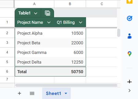
- Step 1: In a new Google Sheets file, enter the following data in A1:B5:
| Project Name | Q1 Billing |
| Project Alpha | 10500 |
| Project Beta | 22000 |
| Project Gamma | 6000 |
| Project Delta | 12250 |
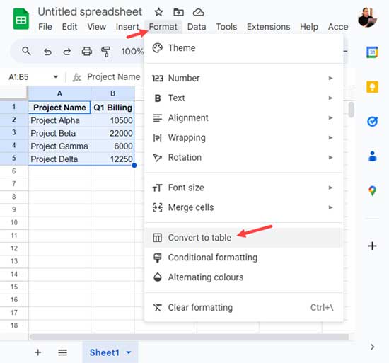
- Step 2: Select the range A1:B5 and click Format > Convert to Table.
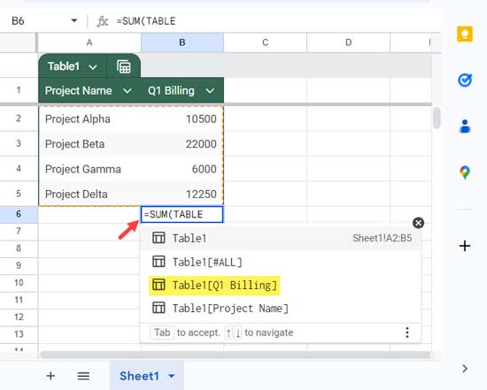
- Step 3: Navigate to cell B6 where you want to apply your formula. Here, we will use the SUM function.
- Step 4: In cell B6, enter
=SUM(TABLEand Google Sheets will list available structured table references.
- Step 5: Select the reference that matches the table name and field label. Based on the sample data, it will be
=SUM(Table1[Q1 Billing]).
- Step 6: Select it and hit enter. This will immediately format the last row as a total row that stands out from the rest of the table with borders.
You can make it more appealing by choosing a different font and making the text bold. Additionally, enter the label “Total” in cell A6.
This is how we can add a total row to a data table in Google Sheets.
Things to Know:
Once you have completed the above steps, adding data below the table will not be included in the table. How do you include them?
- Remove the formula from the total row of the data table. Alternatively, you can delete the row as well.
- Navigate to any cell within the table.
- Click Format > Alternating Colors.
- Uncheck the Footer in the sidebar panel and click Done.
- Click the drop-down next to the table name at the top left corner of the table and select Adjust Table Range.
- Enter the range that includes the new rows, such as A1:B8, in the small window that opens, and click OK.
This will ensure that new data added below the table is included in the table.
Can You Add a Subtotal Row to a Data Table in Google Sheets?
Unfortunately, you cannot directly use structured table references to sum a specific range of rows within a table in Google Sheets.
As a side note, structured references allow you to refer to data within a table using column names instead of cell addresses.
To add subtotal rows within a data table, you should use traditional cell references, but be aware of the following implications:
- The added subtotal rows will move when you apply sorting or column grouping.
- Use the SUBTOTAL function instead of functions like AVERAGE, COUNT, COUNTA, MAX, MIN, PRODUCT, STDEV, STDEVP, SUM, VAR, and VARP in the subtotal rows. Otherwise, when you add a total row to the table at the bottom, these subtotal rows will be included. Also, remember to use the SUBTOTAL function in the total row as well.
Example:
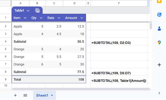
In the following table, assume you want to add a subtotal row below the categories “Apple” and “Orange,” and insert a total row at the end.
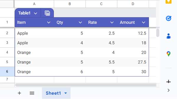
- Right-click on row #3 (the last row in the first category) and select “Insert 1 row below”.
- Right-click on row #7 (the last row in the second category after inserting the above row) and select “Insert 1 row below”.
- In cell D4, enter
=SUBTOTAL(109, D2:D3)to total the first category. The function #109 is used for summing a range. - To get the subtotal for the second category, enter
=SUBTOTAL(109, D5:D7)in cell D8. - Enter
=SUBTOTAL(109, Table1[Amount])in cell D9. - Enter the labels “Subtotal” in cells A4 and A8, and “Total” in cell A9.
- Bold the total and subtotal rows.
Resources
- Dynamic Total Row for FILTER, QUERY, or ARRAY Results in Sheets
- Formula to Insert Group Total Rows in Google Sheets
- Insert Subtotal Rows in a Google Sheets Query Table
- Get the First or Last Row/Column in a New Google Sheets Table
- Customizing Alternating Colors of a Table in Google Sheets
- Structured Table References in Formulas in Google Sheets
- Converting a Range to a Table and Vice Versa in Google Sheets