


The ACCRINT function in Google Sheets calculates the accrued interest of a security, such as a bond, that has periodic coupon payments.
As a side note, the ACCRINTM function in Google Sheets is a similar function. Its purpose is to calculate the accrued interest of a security that pays interest at maturity.
To easily remember the name of this function, use the term ACCRUED INTEREST. The name of the function is derived from the first 4 letters of ACCRUED and the first 3 letters of INTEREST.
Can you explain what accrued interest is?
In simple form, accrued interest is the accumulated interest on a bond since the last interest payment date.
Imagine a bond with a face value of $7,000.00 issued on January 1, 2023, with an interest rate of 4%. The first interest payment is due on July 1, 2023, because the frequency is 2 (the number of interest/coupon payments per year).
If the holder sells the bond beforehand, for example on March 1, 2023, they will receive the interest for the period they held the bond. This interest is known as accrued interest.
Here is a basic formula to calculate the accrued interest:
=(7000 * 0.04 * 60) / 360 // (Par Value * Coupon Rate * Days Accrued) / 360Which will be 46.67.
Although the formula for calculating accrued interest is simple, there are a few reasons why it may be tempting to use the ACCRINT function in Google Sheets. Here are the most important ones:
- The ACCRINT function automatically calculates the accrued days, which can save time and reduce the risk of errors.
- The ACCRINT function can handle different day count conventions, which can be complex to calculate manually.
In addition to these benefits, the ACCRINT function is also more accurate and efficient than manual calculations.
Syntax of the ACCRINT Function in Google Sheets
ACCRINT(issue, first_payment, settlement, rate, redemption, frequency, [day_count_convention])As you can see, out of 7 arguments, 1 is optional, which you can see inside square brackets. Let’s try to understand them one by one.
issue: The issue date of the security.first_payment: The first interest date of the security. (Not in ACCRINTM.)settlement: The settlement date of the security. This is the date after the issue date when the security is traded to the buyer. If the security is held until maturity, the settlement date is the maturity date. In ACCRINTM, this argument will be the maturity date.rate: The annual interest/coupon rate of the security.redemption: The par value. If omitted, the function will assume a par value of $1000.frequency: The number of interest payments per year. (Not in ACCRINTM.) There are three frequencies of coupon payments in the ACCRINT function in Google Sheets that you can choose from:- 1: Annual coupon payment.
- 2: Semiannual coupon payment.
- 4: Quarterly coupon payment.
day_count_convention: (Optional) The day count convention is used to calculate the number of days between the issue date and the settlement date. Day count indicators are listed in the table below.
| Day Count Indicator | Day Count Basis |
| 0 or omitted | US (NASD) 30/360 – As per the National Association of Securities Dealers standard. |
| 1 | Actual/actual |
| 2 | Actual/360 |
| 3 | Actual/365 |
| 4 | European 30/360 – According to European financial conventions. |
How to Use the ACCRINT Function in Google Sheets (with Example)
Here is an example of how to use the ACCRINT financial function in Google Sheets to calculate the coupon payment of security with semi-annual coupon payments:
=ACCRINT(B1,B2,B3,B4,B5,B6,B7)Where:
- B1: Issue date
- B2: First interest date
- B3: Settlement date
- B4: Annual rate of interest
- B5: The par value of the security
- B6: Frequency.
- B7: Day count basis.
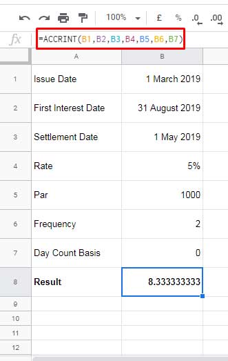
As per the above formula, the accrued interest is 8.33.
When inserting the input values (arguments) directly within the ACCRINT function in Google Sheets, be sure to enter the dates using the DATE function.
Here is the above formula using this approach:
=ACCRINT(DATE(2019,3,1),DATE(2019,8,31),DATE(2019,5,1),5%,1000,2,0)The syntax of the DATE function in Google Sheets is:
DATE(year, month, day)Conclusion
Let’s consider the accrued interest of a bond since the previous coupon payment instead of the principal investment date.
To calculate the accrued interest from the last coupon payment instead of the issue date, set the issue and first_payment arguments to the previous coupon payment date.
Make sure that the settlement date does not fall within the first coupon payment period.
Before we wrap up, one more thing.
If you enter invalid values in the ACCRINT function for accrued interest calculation, the formula will return the following two errors:
- Invalid Date: #VALUE! error.
- Rate/Par
≤0, Invalid Frequency, Invalid Day Count Indicator, or Issue Date≥Settlement Date: #NUM! error.