As part of data analysis, you may need to retrieve the last record from each group in a dataset. This is especially useful when working with time-series data or datasets where events are recorded sequentially. By using a dynamic array formula in Excel, you can automate this process efficiently.

This tutorial will guide you through the process of retrieving the last record in each group in Excel using a dynamic array formula. It also includes a detailed explanation of how the formula works.

Example 1: Retrieve the Last Record in Each Group with Sequential Events

Sample Data:

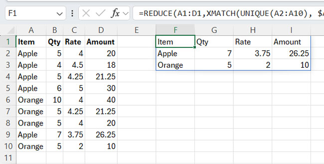
The best way to understand this technique is by using a simple dataset. Consider the following fruit data with columns Item, Qty, Rate, and Amount in the range A1:D10, where A1:D1 contains the headers.

In this case, the Item column is the group column. The goal is to retrieve the most recent purchase details—Qty, Rate, and Amount—for each item.

Formula:

Use the following formula for this dataset:

=REDUCE(
   A1:D1, XMATCH(UNIQUE(A2:A10), A2:A10, 0, -1), 
   LAMBDA(acc, val, VSTACK(acc, FILTER(A2:D10, SEQUENCE(ROWS(A2:A10))=val)))
)

Instructions:

Replace the following ranges in the formula based on your data:

• A1:D1: The header row range.
• A2:D10: The data range (excluding headers).
• A2:A10: The group column range (excluding headers).

The formula assumes the earliest records are at the top and the latest are at the bottom. If your data is reversed, change -1 within the XMATCH function to 1.

If your dataset includes a Date column and you want to extract the latest record, ensure the data is sorted by the Date column in ascending order. Let’s explore this with an example below.

Example 2: Retrieve the Last Record in Each Group for Time Series Data

Sample Data:

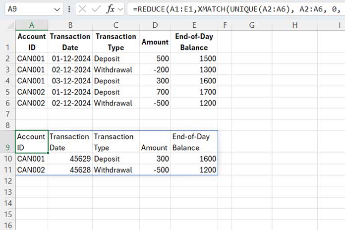
Here’s an example dataset for financial transactions arranged in the following format:

The data range A1:E6 includes the headers Account ID, Transaction Date, Transaction Type, Amount, and End-of-Day Balance.

Steps to Prepare Data:

1. Select the data (A1:E6).
2. Go to the Data tab, and click Sort.
3. Sort by Account ID (A to Z).
4. Add another sort level: Transaction Date (Oldest to Newest).
5. Click OK.

Formula:

To retrieve the last record in each group, use this formula:

=REDUCE(
   A1:E1, XMATCH(UNIQUE(A2:A6), A2:A6, 0, -1), 
   LAMBDA(acc, val, VSTACK(acc, FILTER(A2:E6, SEQUENCE(ROWS(A2:A6))=val)))
)

If the resulting dates appear in a numeric format, apply the Short Date or Long Date format from the Number group in the Home tab.

Note: The formula is identical to the one used in Example 1. The only differences are the references for the data range, group column range, and header row range.

Formula Explanation

The following formula explanation may seem complex to beginners, so it's not necessary to follow this step in detail right away.

The formula combines several powerful Excel functions:

1. UNIQUE(A2:A6): Extracts the unique group values (e.g., Account IDs).
   Result: {"CAN001"; "CAN002"}
2. XMATCH(..., A2:A6, 0, -1): Finds the last occurrence of each unique value in the group column and returns their positions.
   Result: {3; 5}
3. SEQUENCE(ROWS(A2:A6)): Generates a sequence from 1 to the number of rows in the dataset.
   Result: {1; 2; 3; 4; 5}
4. FILTER(A2:E6, SEQUENCE(...) = val): Filters rows corresponding to the positions (named as val) identified by XMATCH. For example:
   • When val = 3, the filter retrieves the third row.
   • When val = 5, it retrieves the fifth row.
   • This ensures only the desired rows (the last record in each group) are included.
5. LAMBDA(acc, val, VSTACK(acc, FILTER(…))): Appends the filtered rows to the accumulated results.
   • The LAMBDA function is a reusable custom formula that processes each value iteratively:
   • acc: The accumulator, starting with the header row (A1:E1).
   • val: The current value in the array returned by XMATCH.
   • VSTACK(acc, ...): Vertically stacks the current result (acc) with the filtered row corresponding to val.
6. REDUCE(...): Iteratively applies the LAMBDA function over the array {3; 5} (positions of the last records) to extract the last record for each group. REDUCE is a LAMBDA helper function in Excel that aggregates results step by step as it processes each element in the input array, producing the final output.

This dynamic approach ensures that you get the correct result even with varying group sizes or data orders.

Conclusion

Retrieving the last record in each group is valuable in various real-world scenarios, such as:

• Sales and Business Reports: Extracting the latest transaction for each customer to analyze their most recent activities.
• Human Resources: Tracking the most recent training session or performance review for each employee.
• Logistics and Supply Chain: Finding the last delivery status for each shipment or package.
• Healthcare: Reviewing the latest medical record or appointment details for each patient in a dataset.
• Event Tracking: Logging the final event in a sequence for each user or process in logs or audits.

This technique not only saves time but also ensures accuracy when dealing with grouped data in Excel, making it an essential tool for analysts and professionals across industries.

Resources

• Lookup Latest Value in Excel and Google Sheets
• Vlookup Last Record in Each Group in Google Sheets
• How to Find the Last Row in Each Group in Google Sheets
• Extract the Earliest or Latest Record in Each Category Based on Timestamp in Google Sheets