You may have records spanning several days and want to filter the last 7 days’ data for sampling or some other purpose. Additionally, the date column may contain either dates or timestamps. Is there a common formula to filter the last 7 days’ data in Excel regardless of whether the column has dates or timestamps?

The answer is yes. But there’s one thing to note. If you want the report to show data from the last 7 days including today as the most current day, you should use one formula. To exclude today, use a different formula.

Formula to Exclude Today’s Date:

=FILTER(filter_range, (INT(date_range) >= TODAY() - 7) * (INT(date_range) < TODAY()))

Formula to Include Today’s Date:

=FILTER(filter_range, (INT(date_range) >= TODAY() - 6) * (INT(date_range) <= TODAY()))

Both formulas are capable of handling dates and datetimes.

How to Use the Formula:

• Replace filter_range with the range you want to filter.
• Replace date_range with the reference to your date column.

Ensure that the filter_range and date_range have the same vertical size because the formula filters based on dates or timestamps in a column.

Example: Filtering Last 7 Days’ Sales Data

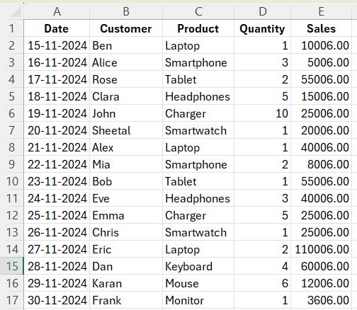
Assume you want to filter the last 7 days’ sales data excluding today from the following sales report spanning A1:E17:

To filter data excluding today, use this formula:

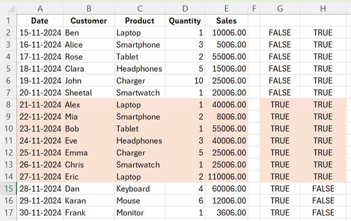
=FILTER(A2:E17, (INT(A2:A17) >= TODAY() - 7) * (INT(A2:A17) < TODAY()))

This will return the records from rows 8 to 14 (as a side note, in our example, today’s date is 28-11-2024).

To filter data including today, use this formula:

=FILTER(A2:E17, (INT(A2:A17) >= TODAY() - 6) * (INT(A2:A17) <= TODAY()))

This will return the records from rows 9 to 15.

Formula Explanation

Let me explain the first formula, which will also help you understand the second one.

The FILTER function in Excel has the following syntax:

FILTER(array, include, [if_empty])

We’ve used the first two arguments:

1. array: A2:E17 – This is the range to filter.
2. include: (INT(A2:A17) >= TODAY() - 7) * (INT(A2:A17) < TODAY()) – Filters rows where the formula evaluates to 1.

This include condition works as follows:

• INT(A2:A17): Removes the time component from datetime values, leaving only the date.
• INT(A2:A17) >= TODAY() - 7: Returns TRUE if the date is greater than or equal to 7 days ago, counting from today. Refer to column G in the following screenshot.
• INT(A2:A17) < TODAY(): Returns TRUE if the date is before today. Refer to column H in the following screenshot.

When these two conditions are multiplied, rows where both conditions are TRUE return 1, while others return 0.

Why Include INT?

If the date column contains timestamps, the INT function ensures that only the date part is evaluated. Without INT, times in the datetime values might prevent accurate filtering.

Resources

• Comparing the FILTER Function in Excel and Google Sheets
• Filter Data from the Previous Month Using a Formula in Excel
• Get Top N Values Using Excel’s FILTER Function
• Search Tables in Excel: Dynamic Filtering for Headers & Data
• Excel: Filter Data with a Dropdown and ‘All’ Option (Dynamic Array)
• How to Apply Nested Column and Row Filters in Excel
• Adding a Dynamic Total Row to Excel FILTER Function Results
• How to Create a Searchable Table in Excel Using the FILTER Function