")
")


")


")

")
")
 in Excel & Google Sheets")


There are two main approaches to fill empty cells with the value from above in Excel. The first option fills empty cells directly within the source data, while the second approach creates a new dataset with filled cells, leaving the original data unchanged.
Both methods are relatively simple. However, the second option is preferable if you are using an Excel version that supports dynamic arrays.
Example Scenario
Consider the following data in the range A1:C13 in an Excel spreadsheet:
| Item | Category | Price |
| Apple | Fruit | 1.5 |
| Orange | Fruit | 1.2 |
| Banana | Fruit | 1 |
| Carrot | Vegetable | 0.8 |
| Tomato | 1.3 | |
| Lettuce | 1.1 | |
| Banana | Fruit | 1 |
| 1 | ||
| 1 | ||
| 1 | ||
| Tomato | Vegetable | 1.3 |
| Tomato | 1.3 |
As you can see, some cells are empty. To fill those empty cells with the values from the cell above, you can use the following methods.
Method 1: The Easiest Way to Fill Empty Cells with the Value from Above
This method directly fills the blanks in the source data.
- Select the range A1:C13 where you want to fill the blanks.
- Press
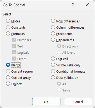
Ctrl + Gto open the Go To dialog box, then click Special. (Alternatively, go to the Home tab, click Find & Select in the Editing group, and select Go to Special.) - In the Go To Special dialog box, select Blanks and click OK.
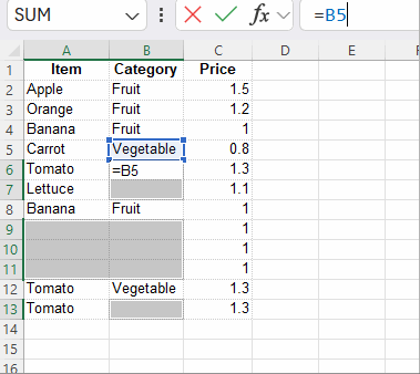
- Now, locate the first blank cell. In our case, it is cell B6.
- Type
=B5in the formula bar to refer to the value from the cell directly above. - Press
Ctrl + Enterto fill all blank cells in the selected range with the values from the cells above.
This method quickly fills all empty cells with the value from the cell directly above.
Note: If this returns formulas instead of values, first select the range and apply the General formatting from the Home tab in the Number group
Method 2: Dynamic Formula to Fill Empty Cells Without Altering Source Data
This approach is useful if you want to keep the original dataset unchanged while filling empty cells in a new dataset.
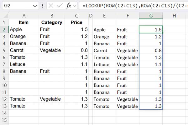
In cell E2 (or a new range where you want the filled data), enter the following dynamic array formula:
=LOOKUP(ROW(A2:A13),ROW(A2:A13)/(A2:A13<>""),A2:A13)This formula will dynamically fill the empty cells in the range A2:A13 with the values from the cells above.
Drag the fill handle from E2 across columns F and G to apply the formula to the other columns (for Category and Price).
Formula Breakdown
Let’s understand how this formula works to fill empty cells with the value from above.
Syntax:
LOOKUP(lookup_value, lookup_vector, result_vector)- We use
ROW(A2:A13)as the lookup_value, which generates a sequence of row numbers (2, 3, … 13). ROW(A2:A13)/(A2:A13<>"")creates an array of row numbers where there are non-blank cells and generates a DIV/0! error in blank rows. This is the lookup_vector.- A2:A13 is the result_vector, the range from which we want to return values.
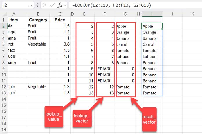
This formula essentially finds the closest previous non-blank cell for each blank cell and returns that value, effectively filling the blank cells with the value from above.
Conclusion
By using either of these two methods, you can efficiently fill empty cells with the value from above in Excel. The first method is quick and straightforward, modifying the original data, while the second method offers a more dynamic approach, leaving the original data unchanged.
Choose the method that best suits your needs depending on whether you want to modify the source data or create a new filled dataset.