You can easily insert subtotals using a dynamic array formula in Excel. Why use this approach when Excel already provides built-in options?

Built-in Options for Inserting Subtotals in Excel

Excel offers tools like Pivot Tables (from the Insert tab) and the Subtotal option (from the Data tab, Outline group) to insert subtotals.

However, these tools have some limitations:

• The Subtotal function requires your data to be sorted and applies changes directly to the source data.
• With Pivot Tables, while powerful, they can be cumbersome to maintain and may not retain your preferred formatting.

Benefits of Using a Dynamic Array Formula for Inserting Subtotals

Using a dynamic array formula for inserting subtotals in Excel has several advantages:

1. No modification to source data: The original data remains unchanged, and there is no need to sort it.
2. Preserves formatting: Subtotals are added as new rows without affecting the formatting of your source data.
3. Flexible functions: You can apply different functions like SUM, AVERAGE, MIN, and MAX to subtotals.
4. Customizable subtotal rows: You can choose to display only the subtotal rows if needed.
5. Specific columns: You can add subtotals for specific columns.
6. Custom grouping: You can specify any column to group your data by.

Prerequisites

To use the dynamic array formula for inserting subtotals:

• You need at least two columns:
  • The first column will not be included in the calculations, as it will be used to display the labels (e.g., “…, Total”)
  • The second (or more) will be used for applying functions like SUM.

Dynamic Array Formula for Inserting Subtotals

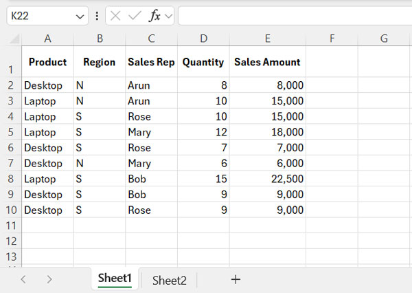
Consider the following sample data in A1:E10 in Sheet1:

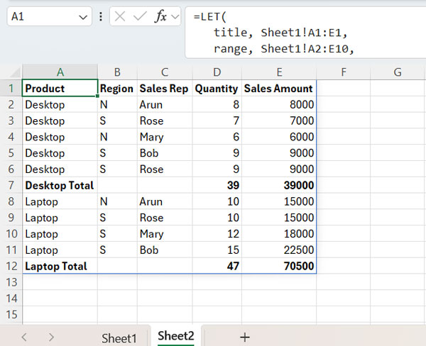
You can insert the following formula in cell A1 of Sheet2 (or any other sheet in the same workbook):

=LET(
   title, Sheet1!A1:E1,
   range, Sheet1!A2:E10,
   total_col, {4, 5},
   group_col, 1,
   IFNA(
      REDUCE(
         title, TOCOL(UNIQUE(CHOOSECOLS(range, group_col)), 3),
         LAMBDA(acc,val,
            LET(
               total1, FILTER(range, CHOOSECOLS(range, group_col)=val),
               total2, HSTACK(val&" Total", BYCOL(FILTER(CHOOSECOLS(range, SEQUENCE(COLUMNS(title)-1, 1, 2)),CHOOSECOLS(range, group_col)=val), LAMBDA(col, SUM(col)))),
               matching, XMATCH(SEQUENCE(1, COLUMNS(title)), HSTACK(1, total_col)),
               VSTACK(acc, total1, IF(matching, total2, ""))
            )
         )
      ), ""
   )
)

Formula Customization

To adapt this formula for your dataset, follow these steps:

1. Replace Sheet1!A1:E1 (title) with the reference to your header row.
2. Replace Sheet1!A2:E10 (range) with your data range, excluding the header row.
   • Ensure the number of columns in the title and range match.
3. Replace the array constant {4, 5} with the column numbers where you want to apply subtotals. For example, use {5} to total the fifth column, or {2, 3, 5} to total the second, third, and fifth columns.
4. Replace 1 (group_col) with the column number by which you want to group the data (e.g., 1 for “Product,” 3 for “Sales Rep”).
5. Feel free to replace the SUM function with AVERAGE, MIN, MAX, COUNT, or COUNTA.

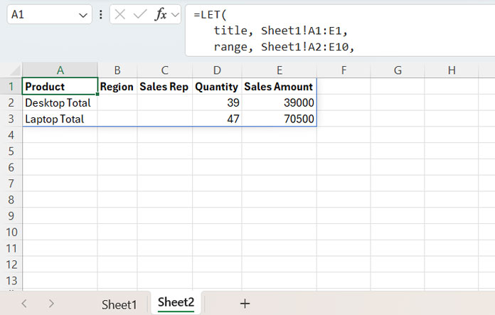
How to Extract Subtotal Rows Only

If you only want to display the subtotal rows, modify this part of the formula:

Replace:

VSTACK(acc, total1, IF(matching, total2, ""))

With:

VSTACK(acc, IF(matching, total2, ""))

This will exclude the original data rows and only display the subtotal rows, providing a summary view.

Formula Breakdown

The formula inserting subtotals in Excel is built around the REDUCE function, which takes an initial value and an array, and then applies a LAMBDA function to each element in the array. An accumulator stores the result and stacks the intermediate results.

Syntax: REDUCE(initial_value, array, function)

• initial_value: title (A1:E1) represents the header row.
• array: TOCOL(UNIQUE(CHOOSECOLS(range, group_col)), 3) retrieves the unique values in the grouping column.

Function Components:

• total1: Filters the data based on each unique group value:

FILTER(range, CHOOSECOLS(range, group_col)=val)

• total2: Horizontally stacks the group name with the subtotal of each numeric column, except the first column:

HSTACK(val & " Total", BYCOL(FILTER(CHOOSECOLS(range, SEQUENCE(COLUMNS(title)-1, 1, 2)), CHOOSECOLS(range, group_col)=val), LAMBDA(col, SUM(col))))

It returns the subtotal row.

• matching: Identifies the columns to apply the subtotal (SUM, AVERAGE, …) function:

XMATCH(SEQUENCE(1, COLUMNS(title)), HSTACK(1, total_col))

• Final output: VSTACK(acc, total1, IF(matching, total2, "")) vertically stacks the accumulator with the filtered data (total1) and the subtotals (total2), if applicable. The IF logical test ensures that totals appear in the specified columns (total_col) along with the corresponding total labels.

Resources

• Adding a Dynamic Total Row to Excel FILTER Function Results
• Grouping and Subtotals in Google Sheets and Excel
• Formula to Insert Group Total Rows in Google Sheets
• Insert Subtotal Rows in a Google Sheets Query Table
• Dynamic Total Row for FILTER, QUERY, or ARRAY Results in Sheets