


")


")

")
")
 in Excel & Google Sheets")


When highlighting parent and child rows or columns, I mean applying conditional formatting to adjacent cells. How can this be done in Excel?
For example, you might want to check the value in one cell and highlight that cell along with the next cell, which are in two different rows. This is particularly useful when you have a title row followed by a value row, creating multiple pairs of rows.
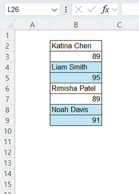
Table 1:
| Katina Chen |
| 89 |
| Liam Smith |
| 95 |
| Rimisha Patel |
| 89 |
| Noah Davis |
| 91 |
In another scenario, you may want to check the value in one cell and highlight that value along with the next value in an adjacent column.
Table 2:
| Katina Chen | 89 | Liam Smith | 95 | Rimisha Patel | 99 | Noah Davis | 91 |
Let’s see how to create a new rule for this in Excel using Conditional Formatting.
Example of Highlighting Parent and Child Rows in Excel
Assume the names in Table #1 above are in the range B2:B9 in an Excel spreadsheet. We will highlight the names in one row and their marks in another row if the mark is greater than 90.
Here are the steps you should follow to highlight two adjacent cells in an Excel spreadsheet:
- Select the range B2:B9.
- Navigate to the Home tab, and under the Styles group, click Conditional Formatting > New Rule.
- In the New Formatting Rule dialog box that opens, select “Use a formula to determine which cells to format.”
- Enter the following formula in the provided field:
=OFFSET(B2, MOD(ROW(A1), 2),)>90 - Click the Format button and choose a formatting style, preferably a fill color other than white.
- Click OK to close the Format Cells dialog box, and then click OK again to close the New Formatting Rule dialog box.
This will highlight the names and marks of those whose marks are greater than 90.
This is an example of how to highlight parent and child rows in Excel.
Note: When you use this formula in your Excel spreadsheet for a different range, simply replace B2 with the cell reference of the first value in the column (the top-left cell in the range if you are applying it in a 2D array).
Example of Highlighting Parent and Child Columns in Excel
If you refer to the second table, you can see that the data in the example above is arranged in a row. Therefore, we need to highlight two adjacent columns that meet the criterion in one column.
Assume the range is B2:I2.
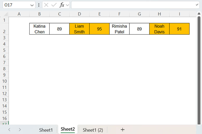
You can follow all the steps from the previous example, but in the first step, you should select the range B2:I2, and in the fourth step, you should use the following formula: =OFFSET(B2, 0, MOD(COLUMN(A1), 2))>90
This will help us highlight parent and child columns in Excel. The “Note” from the previous example applies here as well.
How Do the Formulas Highlight Linked Data in Adjacent Cells?
Both Excel highlight rules use the OFFSET function to offset rows or columns based on the orientation of the data.
The formula for Table #1 offsets one row in the title row to fetch the mark. In the rows with marks, it offsets zero rows. Essentially, the formula evaluates the marks in each row, and if they are greater than 90, the highlighting is applied.
If you enter MOD(ROW(A1), 2) in any cell and drag it down, it will generate an array of values such as {1; 0; 1; 0; 1; 0; …}. These values are used to offset the rows in each case.
The same applies to the second conditional formatting rule, where we used the COLUMN function instead of the ROW since we are applying the rule to columns and offsetting columns, not rows.