


")


")

")
")
 in Excel & Google Sheets")


You may have data arranged in a column with categories followed by subcategories. In this case, you might want to extract the subcategories between two categories or move subcategories to different columns. We can refer to this as extracting rows between two texts. How do we do that in Excel?
If you’re using an older version of Excel, you can use an INDEX-MATCH combo. If you have a version of Excel that supports XLOOKUP and dynamic arrays, you’re in luck. While you can still use the INDEX-MATCH combo, you can replace it with XLOOKUP for a more efficient solution. Plus, you can apply this method to all categories and subcategories in a column in one go. For that, we’ll use a combination of REDUCE and XLOOKUP.
How to Extract All Rows Between Two Texts in a Column in Excel
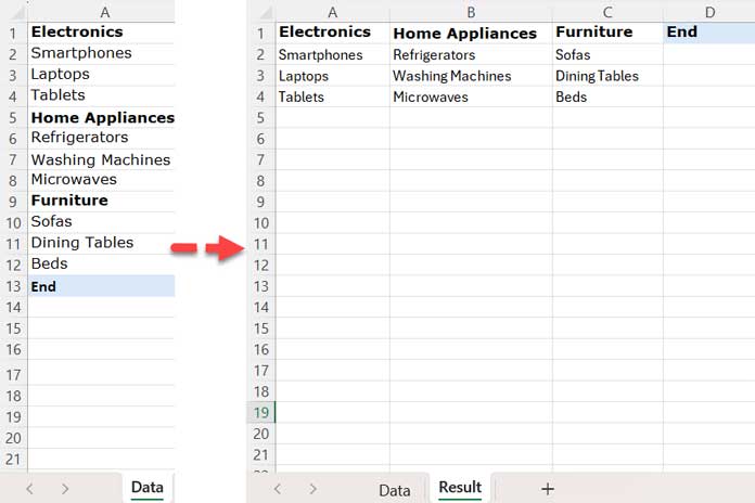
Assume you have the following sample data in column A of an Excel spreadsheet, on the sheet named ‘Data’:
| Electronics |
| Smartphones |
| Laptops |
| Tablets |
| Home Appliances |
| Refrigerators |
| Washing Machines |
| Microwaves |
| Furniture |
| Sofas |
| Dining Tables |
| Beds |
In the second sheet, named ‘Result,’ you want to extract the rows between two texts, such as ‘Electronics’ and ‘Home Appliances.’
- In the ‘Result’ sheet, enter ‘Electronics’ in cell A1 and ‘Home Appliances’ in cell B1.
- Then, in cell A2, enter the following formula:
=INDEX(Data!$A:$A,MATCH(A1,Data!$A:$A,0)+1):INDEX(Data!$A:$A,MATCH(B1,Data!$A:$A,0)-1) - In older versions of Excel, you’ll need to enter this formula as an array formula by pressing Ctrl + Shift + Enter instead of just Enter.
If you want to move all subcategories to their corresponding columns:
- Enter all the category names in row 1 of the ‘Result’ sheet.
- Drag the formula across the row to fill in the subcategories.
Before doing that, navigate to the last non-blank cell in column A of the ‘Data’ sheet and enter the text “end” in the cell below it. In the ‘Result’ sheet, enter “end” in the first row after the last category. (Please scroll up to see the screenshot).
Then, drag the formula in A2 across the row. This will allow you to move all subcategories into their respective columns under the corresponding categories.
Do you need to use the text “end”? No, you can use any text or character. Just ensure you use the same text or character in both the ‘Data’ and ‘Result’ sheets.
Formula Breakdown
This section is optional; you can skip it if you prefer.
INDEX(Data!$A:$A,MATCH(A1,Data!$A:$A,0)+1): Returns the cell at the specified row position based on the row number determined.MATCH(A1, Data!$A:$A, 0) + 1: Finds the row position of the first text in the column and adds 1 to determine the start of the range.
INDEX(Data!$A:$A,MATCH(B1,Data!$A:$A,0)-1): Returns the cell at the specified row position based on the row number determined.MATCH(B1, Data!$A:$A, 0) - 1: Finds the row position of the second text in the column and subtracts 1 to determine the end of the range.
The range operator (:) between the two INDEX-MATCH formulas creates a range that includes all rows (subcategories) between the two texts (categories), excluding the headings.
This is one way to extract rows between two texts in Excel. If you are using newer versions of Excel that support XLOOKUP and dynamic arrays, you can use the following formula as well.
Dynamic Array Formula for Extracting Rows Between Texts in Excel
You won’t encounter any issues extracting rows between two texts using the formula provided in the latest versions of Excel.
However, when dealing with several categories and subcategories in a column and moving all subcategories to their relevant category columns, you can use the following approach.
Earlier, we dragged the formula in cell A2 across the row in the Result sheet. Now, simply enter the following formula in cell A2, and it will handle the rest:
=IFNA(DROP(
     REDUCE("", A1:C1, LAMBDA(accu, val,
        LET(
            titleA, val, titleB, OFFSET(val, 0, 1),
            data,
               XLOOKUP(titleA, Data!A:A, Data!A:A):
               XLOOKUP(titleB, Data!A:A, Data!A:A),
            HSTACK(accu, FILTER(data, (data<>titleA)*(data<>titleB)*(data<>"")))
        )
     )), 0, 1
), "")
In this formula, A1:C1 refers to the category range in the ‘Result’ tab, and Data!A:A is the source data.
You should also enter the text “End” in both the ‘Data’ and ‘Result’ tabs as mentioned earlier.
If you want to extract rows between two texts, replace A1:C1 in the formula with A1:B1.
Formula Explanation
The formula uses several advanced Excel functions, including LAMBDA, REDUCE, XLOOKUP, and HSTACK. If this explanation seems complex, you may choose to skip it.
REDUCE("", A1:C1, LAMBDA(accu, val, ...)):
REDUCE: This function iterates through each element of the arrayA1:C1. It starts with an initial value of""(an empty string) for the accumulator (accu).LAMBDA(accu, val, ...): This lambda function defines how each iteration ofREDUCEwill process.accurepresents the accumulated result so far, andvalis the current element from the arrayA1:C1.
Inside LAMBDA:
LET(titleA, val, titleB, OFFSET(val, 0, 1), ...):titleA: Assigned the value ofval, which is the current element in the arrayA1:C1.titleB: Assigned the value of the cell immediately to the right ofval, obtained usingOFFSET(val, 0, 1).
data:XLOOKUP(titleA, Data!A:A, Data!A:A):XLOOKUP(titleB, Data!A:A, Data!A:A): This creates a range reference between the rows corresponding totitleAandtitleBin column A of theDatasheet.
FILTER(data, (data<>titleA)*(data<>titleB)*(data<>"")):FILTER: Filters thedatato excludetitleA,titleB, and any blank cells.
HSTACK(accu, ...):HSTACK: Horizontally stacks the filtered results from the current iteration onto the accumulated results.
Result:
- The
REDUCEfunction iterates through each pair of headings inA1:C1, extracts the subcategories between each pair, and stacks them horizontally into the final result.
The formula stacks columns of varying lengths, which may result in #N/A cells being added to match the number of rows across columns. The IFNA function handles these #N/A cells by replacing them with empty cells. Finally, the DROP function removes the extra empty column added at the beginning of the result.
Can I Use These Formulas in Google Sheets?
The INDEX-MATCH formula will work in Google Sheets. However, the dynamic array formula described above won’t work in Google Sheets because it currently lacks the DROP function. Instead, Google Sheets offers a better option using the MAP and LAMBDA functions. You can explore this alternative in Filter Values Between Two Headings in Google Sheets. Unfortunately, this formula won’t work in Excel, so we need to use two separate approaches: one for Excel and one for Google Sheets.
Resources
- Highlight Groups with Alternating Colors in Excel
- Excel: Calculating Cumulative Sum by Group
- Combine Two Tables in Excel Using a Dynamic Array Formula
- Search Tables in Excel: Dynamic Filtering for Headers & Data
- Unpivot Excel Data Fast: Power Query & Dynamic Array Formula
- Flip a Table Vertically in Excel (Includes Dynamic Array Formula)