In Excel, you can calculate the cumulative sum by group using a regular drag-down formula or a dynamic array formula if your Excel version supports it.
Both formulas use the SUMIF function, but for the dynamic array formula, we will use the MAP function additionally.
Formulas to Calculate Cumulative Sum By Group in Excel
Non-Array Formula:
=SUMIF($A$2:A2, A2, $B$2:B2)This formula in cell C2 assumes column A contains the category and column B contains the amount to sum.
Drag this formula from cell C2 as far as you need.
Array Formula:
=MAP(A2:A10,B2:B10,LAMBDA(group,amount,SUMIF(A2:group,group,B2:amount)))This formula takes the category range A2:A10 and the amount range B2:B10. Clear the range C2:C10 and enter this formula in cell C2. You can edit the ranges to include all records, like A2:A100 and B2:B100, but both should be of the same size.
Let’s see examples of calculating the cumulative sum by group using the above array and non-array formulas in an Excel spreadsheet.
Examples of Cumulative Sum by Group
I have the following fruit data in A2:AB0 in an Excel spreadsheet:
| apple | 5 |
| apple | 10 |
| apple | 5 |
| apple | 5 |
| orange | 6 |
| orange | 6 |
| orange | 10 |
| orange | 6 |
| orange | 5 |
Non-Array Formula:
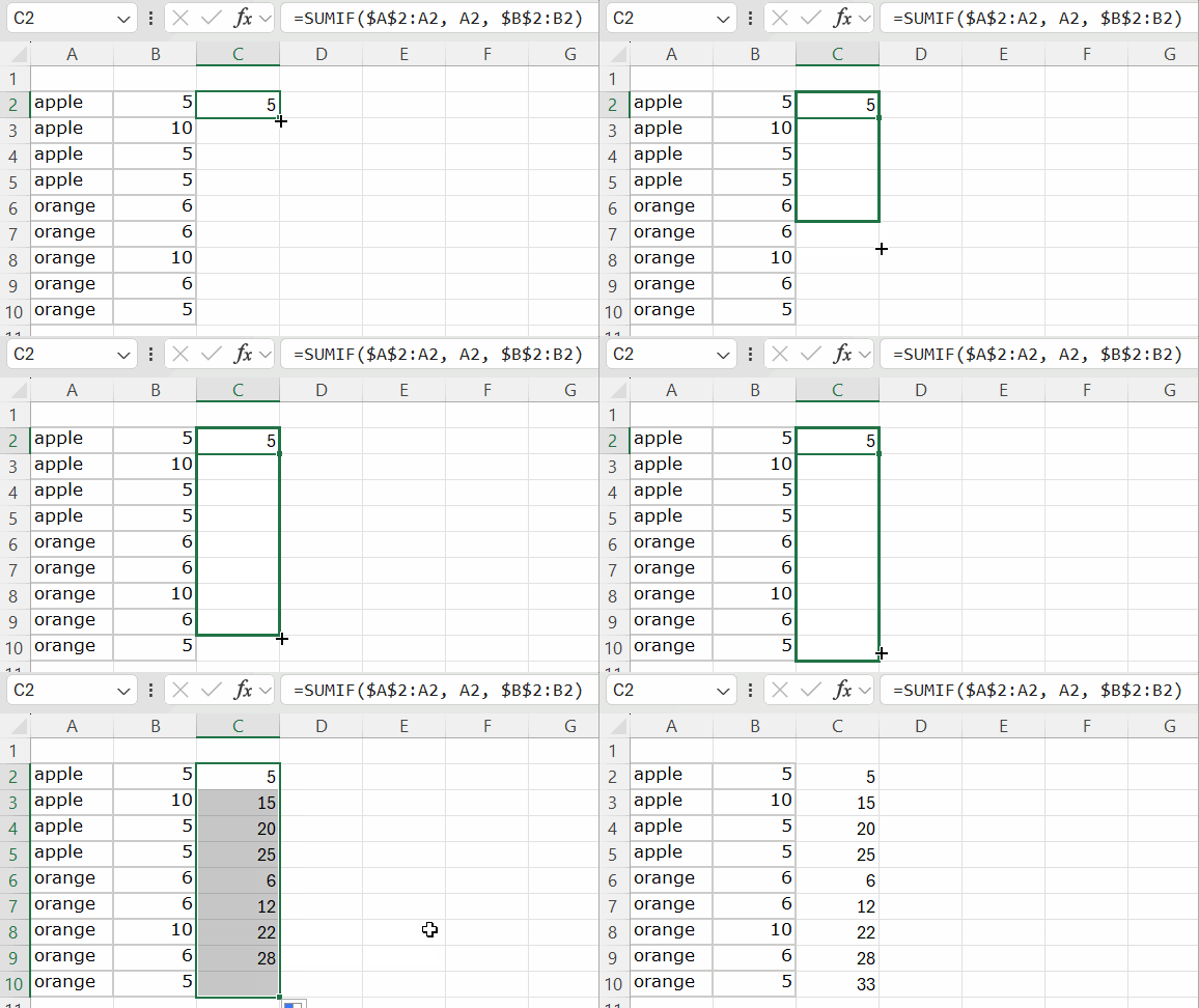
- In cell C2, enter the following non-array formula:
=SUMIF($A$2:A2, A2, $B$2:B2) - Navigate to cell C2, if not already there.
- Point your mouse at the bottom right corner of cell C2 until it turns into a + sign.
- Click and drag down to cell C10.

There are two groups in the above example: “apple” and “orange”.
- The amounts for “apple” are 5, 10, 5, and 5, so the running total will be 5, 15, 20, and 25.
- The amounts for “orange” are 6, 6, 10, 6, and 5, so the running total for this group will be 6, 12, 22, 28, and 33.
The difference between a cumulative sum and a group-wise cumulative sum is that the latter resets whenever the group changes in a column.
As a side note, the above Excel formulas will work even if the values in the category column (A2:A10) are not sorted.
Array Formula:
The array formula will return the same output, but you don’t need to drag it down from C2. It will spill the results from cell C2 down to C10, provided C3:C10 is empty:
=MAP(A2:A10,B2:B10,LAMBDA(group,amount,SUMIF(A2:group,group,B2:amount)))Note: This will only work in Excel versions that support the MAP and LAMBDA functions.
Explanation of the Formulas
We use the SUMIF function to sum a column based on a condition in another column.
Typically, we use ranges like A2:A10 (criteria range) and B2:B10 (sum range). However, in this case of group-wise cumulative sum, we use dynamic ranges such as $A$2:A2 and $B$2:B2 so that we get the total up to the current row as we drag it down. These ranges become $A$2:A3 and $B$2:B3 in the next row and increase accordingly.
The same logic is automated using the MAP function, where we specify the arrays A2:A10 and B2:B10 and name the current elements ‘group’ and ‘amount’.
We then use the ranges A2:group and B2:amount in SUMIF. The MAP function maps each element in the array and returns the group-wise cumulative sum.


