You can use a dynamic array formula to calculate weekly averages in Excel without relying on helper columns.

To calculate weekly averages, you typically have a date column and an amount column and want to find the weekly average of the amounts.

Assume you have data in A1:B65 with dates in column A and amounts in column B, where A1:B1 contains the field labels. To calculate the weekly average from this data, you would typically follow these three steps:

1. Extract Week Numbers (Helper Column 1):

Enter the following formula in cell D2 and drag it down to D65:

=WEEKNUM(A2, 2)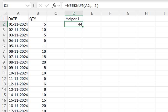

Here, 2 is the return_type, representing a Monday week start. You can choose one of the following instead:

• 1: Week starts on Sunday.
• 2: Week starts on Monday (as used in the formula above).
• 11-17: Custom week starting days (Monday to Sunday).

There is one more return_type, which is 21. I don’t recommend using it if you have data that spans across the year. This type follows the ISO 8601 standard, where week #1 starts on Monday and is defined as the week containing the first Thursday of the year.

2. Extract Years (Helper Column 2):

Enter the following formula in cell E2 and drag it down to E65:

=YEAR(A2)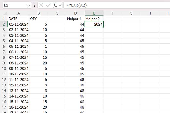

3. Calculate the Weekly Average:

Finally, use the following AVERAGEIFS formula in cell F2 and drag it down to F65 to calculate the weekly average:

=IF((D2=D1)*(E2=E1),"",AVERAGEIFS($B$2:$B$65,$D$2:$D$65,D2,$E$2:$E$65,E2))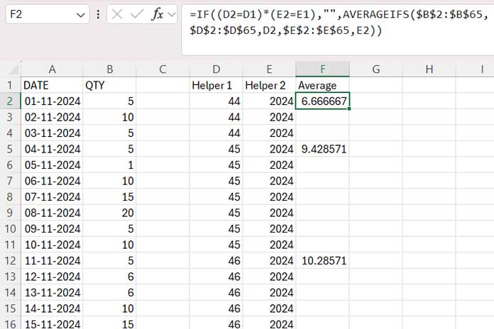

Dynamic Weekly Averages in Excel Without Helper Columns: Challenges and Solution

Challenges

In Excel, avoiding helper columns in dynamic weekly average calculations can be tricky because you may need to nest LAMBDA helper functions like MAP to achieve the same result. Unfortunately, nesting AVERAGEIF or AVERAGEIFS won’t work, resulting in a #CALC! error with a tooltip that says “Nested arrays are not supported.“

So, even though a formula that works in Google Sheets for dynamic weekly averages may not work in Excel, you can find a way to replace AVERAGEIF/AVERAGEIFS with SUMPRODUCT. I’ve addressed this in my formula below.

Solution

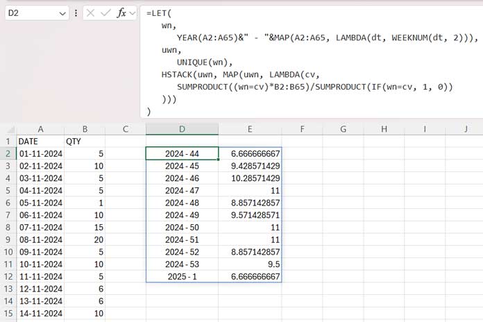
You can use the following dynamic array formula in Excel to calculate weekly averages:

=LET(
   wn, 
      YEAR(A2:A65)&" - "&MAP(A2:A65, LAMBDA(dt, WEEKNUM(dt, 2))), 
   uwn, 
      UNIQUE(wn), 
   HSTACK(uwn, MAP(uwn, LAMBDA(cv, 
      SUMPRODUCT((wn=cv)*B2:B65)/SUMPRODUCT(IF(wn=cv, 1, 0))
   )))
)

In this formula, replace A2:A65 with your date column range and B2:B65 with your amount column range.

Additionally, you can adjust the return_type value from 2 (which represents a Monday week start, as explained above) to fit your preferred week start day.

This formula doesn’t rely on helper columns and returns the weekly averages dynamically.

Formula Explanation

You can skip this formula explanation if it seems complex, especially for basic users.

I used the LET function to assign names to calculation results within the dynamic average formula, allowing these named values to be reused multiple times in the same formula.

Syntax:

LET(name1, name_value1, [name2, …], [name_value2, …], formula_expression)

The names are wn, uwn, and the formula expression starts with HSTACK.

• wn (representing week numbers): YEAR(A2:A65)&" - "&MAP(A2:A65, LAMBDA(dt, WEEKNUM(dt, 2)))
  This part combines the year from A2:A65 with the week number. The YEAR function returns an array of years, while WEEKNUM needs the MAP LAMBDA function to generate an array of week numbers. Google Sheets can handle WEEKNUM without additional helper functions, but Excel requires MAP here.
• uwn (representing unique week numbers): UNIQUE(wn)
  This returns the unique week numbers from the wn array.

Formula Expression:

HSTACK(uwn, MAP(uwn, LAMBDA(cv, 
      SUMPRODUCT((wn=cv)*B2:B65)/SUMPRODUCT(IF(wn=cv, 1, 0))
   )))

It consists of three parts:

1. SUMPRODUCT((wn=cv)*B2:B65)
   Returns the sum of amounts in B2:B65 where the week number (wn) matches the current unique week number (cv).
2. SUMPRODUCT(IF(wn=cv, 1, 0))
   The IF function returns 1 if the week number (wn) matches the current unique week number (cv). SUMPRODUCT then totals these values to give the count.
3. Part 1 / Part 2
   This calculates the weekly average for the current unique week number.

The MAP function iterates through each element in uwn to generate a dynamic weekly summary, which is horizontally appended to uwn using HSTACK.

Dynamic Weekly Averages with a Custom Function in Excel

We aim to help you calculate weekly averages in Excel without using helper columns. The dynamic array formula provided achieves this.

Creating a custom function can save time and effort in calculating dynamic weekly averages across multiple spreadsheets.

Here’s how to create a custom function:

1. Click the Formulas tab.
2. Under the Defined Names group, select Name Manager.
3. Click New in the window that opens.
4. In the Name field, enter WEEKLY_AVERAGE.
5. Under Scope, choose Workbook if it’s not already selected.
6. In the Refers to field, replace any existing formula with the following formula:
   =LAMBDA(average_range,criteria_range, LET( wn, YEAR(criteria_range)&" - "&MAP(criteria_range, LAMBDA(dt, WEEKNUM(dt, 2))), uwn, UNIQUE(wn), HSTACK(uwn, MAP(uwn, LAMBDA(cv, SUMPRODUCT((wn=cv)*average_range)/SUMPRODUCT(IF(wn=cv, 1, 0)) ))) ))
7. Click OK.
8. Close the Name Manager.

You can then use the following function for dynamic weekly averages in that workbook:

Syntax:

WEEKLY_AVERAGE(average_range, criteria_range)

For the sample data provided, the formula would be:

=WEEKLY_AVERAGE(B2:B65, A2:A65)

Resources

• Sum by Week Number in Excel (Dynamic Array Formula Included)
• Dynamic Moving Average in Excel