To sum every 7 rows, you can use either a drag-down formula or a dynamic array formula in Excel. This method is especially useful when you want to calculate weekly totals in a column that contains data entered in chronological order.

How to Use a Drag-Down Formula to Sum Every 7 Rows in Excel

If you prefer a drag-down formula, which is undoubtedly the simplest option, try this:

=SUM(OFFSET(range_start, (ROW(A1)-1)*7, 0, 7, 1))

Replace range_start with the starting cell reference in absolute reference format (e.g., $B$2). No other changes are required.

Example:

Assume you have dates in column A (A2:A) and corresponding sales data in column B (B2:B). To calculate weekly totals, use the following formula in cell C2 and drag it down:

=SUM(OFFSET($B$2, (ROW(A1)-1)*7, 0, 7, 1))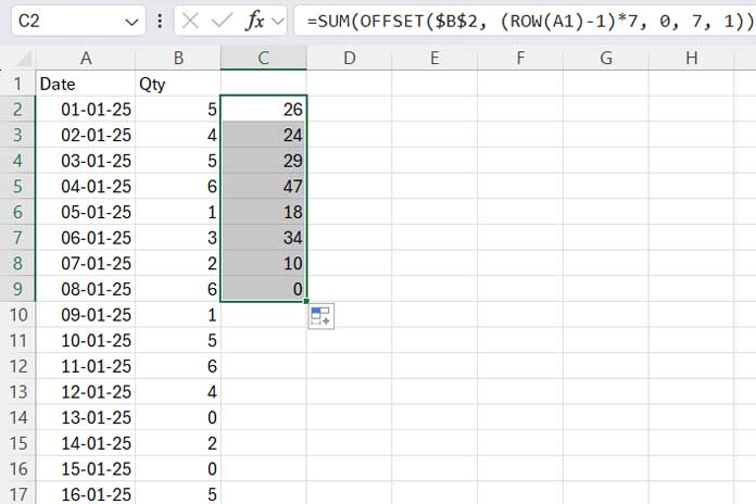

When applying this formula to a different dataset, replace $B$2 with the first cell reference of your range. You can leave A1 unchanged.

How the Formula Works:

The OFFSET function dynamically adjusts the range it sums based on the row number. The syntax is as follows:

=OFFSET(reference, rows, cols, [height], [width])

• reference: $B$2 (starting cell of the range).
• rows: (ROW(A1)-1)*7 (adjusts the starting point to sum every 7 rows: 0 rows, then 7 rows, then 14 rows, and so on).
• cols: 0 (no column offset, stays in column B).
• height: 7 (sums 7 rows at a time).
• width: 1 (sums a single column).

Create a Dynamic Array Formula to Automatically Sum Every 7 Rows

If you want to sum every 7 rows in one go, use the MAP function, one of Excel’s powerful LAMBDA-based functions.

Example:

If the data is in B2:B50, enter this formula in cell C2:

=MAP(
   SEQUENCE(ROUNDUP(ROWS(B2:B50)/7, 0), 1, 2, 7), 
   LAMBDA(x, SUM(FILTER(B2:B50, (ROW(B2:B50)>=x)*(ROW(B2:B50)<=x+6))))
)

Using this formula to sum every 7 rows is simple. You just need to replace all occurrences of B2:B50 with your actual data range and adjust the number 2 (row number where the range starts) as needed. However, understanding the formula might seem complex because it involves nested functions like MAP and LAMBDA. Let’s break it down.

Formula Breakdown:

MAP Syntax:

=MAP(array1, lambda)

• array1: The input array on which the LAMBDA function operates.
• lambda: A custom function applied to each element in array1.

In Our Formula:

• array1: SEQUENCE(ROUNDUP(ROWS(B2:B50)/7, 0), 1, 2, 7)
  • Generates sequence numbers with a step value of 7, corresponding to the starting row of each 7-row block (e.g., {2; 9; 16; 23; 30; 37; 44}).
• lambda: LAMBDA(x, SUM(FILTER(B2:B50, (ROW(B2:B50)>=x)*(ROW(B2:B50)<=x+6))))
  • For each x in array1:
    • FILTER(B2:B50, (ROW(B2:B50)>=x)*(ROW(B2:B50)<=x+6)): Filters rows between x and x+6.
    • SUM: Totals the filtered rows.

In short, the MAP function applies the LAMBDA to each element in array1, returning the total of every 7 rows.

Resources

• Sum by Week Number in Excel (Dynamic Array Formula Included)
• Dynamic Weekly Averages in Excel Without Helper Columns