This tutorial explains how to duplicate rows based on cell values in a column without relying on VBA in Excel. All you need is a version of Excel that supports dynamic arrays.
For this purpose, we will use functions such as ROWS, SEQUENCE, REPT, TEXTJOIN, TEXTSPLIT, TOCOL, and CHOOSEROWS.
If your version of Excel supports these functions, you can proceed without any further ado. The formula does not use LAMBDA functions, so the performance of the formula won’t be affected.
Core Idea Behind Duplicating Rows
The core concept of duplicating rows based on cell content is as follows:
We will use a single row to explain how to duplicate rows based on quantity.
| Title | Author | Qty |
| To Kill a Mockingbird | Harper Lee | 3 |
In this data, Title contains the book title, Author contains the author name, and Qty specifies the quantity (in this case, 3).
The goal is to repeat the book title and author name based on the quantity (i.e., 3) as follows:
| Title | Author |
| To Kill a Mockingbird | Harper Lee |
| To Kill a Mockingbird | Harper Lee |
| To Kill a Mockingbird | Harper Lee |
Here’s how we’ll achieve this:
- We assign a serial number to the row. We number it #1 since it’s the first row (record) in the table.
- Next, we repeat this serial number 3 times, corresponding to the quantity.
- These numbers can then be used in the CHOOSEROWS function to return the first row 3 times, like so:
=CHOOSEROWS(row, {1, 1, 1}).
However, when there are multiple rows, we need to generate various serial numbers dynamically to use with CHOOSEROWS. We will cover how to generate these serial numbers in the step-by-step guide below. Before that, let’s dive into the formula for dynamically duplicating rows based on cell content in Excel.
Dynamic Array Formula for Duplicating Rows Based on Cell Values in Excel
You can use the following formula to repeat rows based on cell contents in Excel:
=CHOOSEROWS(
   A2:B5,
   TOCOL(
      TEXTSPLIT(
         TEXTJOIN("", TRUE,
            REPT(SEQUENCE(ROWS(C2:C5))&"|", C2:C5)
         ), "|"
      )*1, 3)
   )
In this formula, replace A2:B5 with your range of rows to be repeated, and C2:C5 with the cell range that determines how many times each row should be repeated.
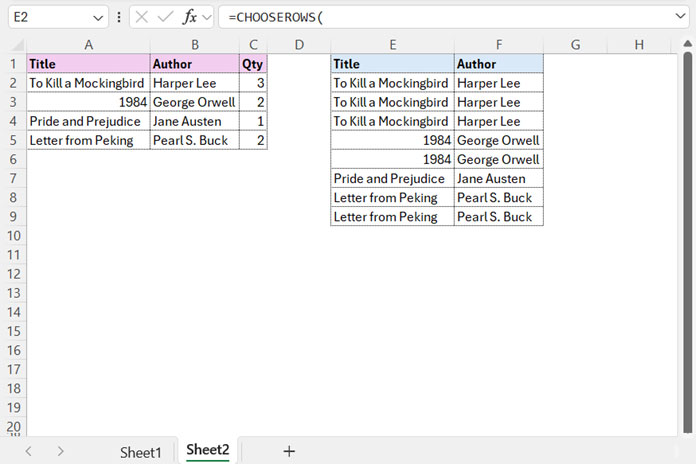
The formula in cell E2 produces the following output:

Formula Explanation
The formula above follows a straightforward logic, which we have already discussed under the subtitle “Core Idea Behind Duplicating Rows”.
Below is a step-by-step explanation to help you use the formula correctly and learn some new techniques in Excel.
Step 1: Prepare the Sample Data for Duplicating Rows Based on Cell Content
When duplicating data, ensure that the column determining the number of rows to duplicate is the last one. If it’s in the middle, additional steps may be required to exclude it from the new table generated by the formula.
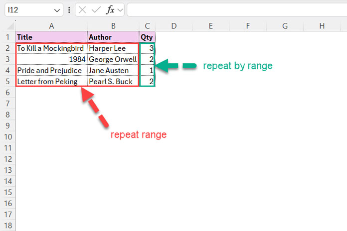
Here is the correct format:

- Repeat range: A2:B5
- Repeat by range: C2:C5
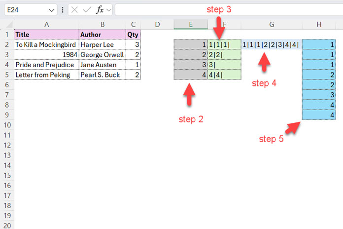
Step 2: Assign Serial Numbers
To assign serial numbers to the duplicate row range, use the following formula:
=SEQUENCE(ROWS(C2:C5))
Step 3: Repeat Serial Numbers
The following formula repeats the serial numbers based on the values in C2:C5 and inserts a “|” delimiter between them:
=REPT(SEQUENCE(ROWS(C2:C5)) & "|", C2:C5)Step 4: Join the Repeated Serial Numbers
Use the TEXTJOIN function in Excel to join the repeated serial numbers as follows:
=TEXTJOIN("", TRUE, REPT(SEQUENCE(ROWS(C2:C5)) & "|", C2:C5))Step 5: Split and Arrange Serial Numbers into a Column
This step is crucial for duplicating rows based on cell content in Excel.
=TOCOL(TEXTSPLIT(TEXTJOIN("", TRUE, REPT(SEQUENCE(ROWS(C2:C5)) & "|", C2:C5)), "|") * 1, 3)The TEXTSPLIT function splits the joined serial numbers based on the pipe delimiters. Since the result is text, we multiply by 1 to convert them back to numeric values. The TOCOL function arranges the values into a column and removes any error values.
Step 6: Use CHOOSEROWS to Duplicate Rows Based on Cell Content
The formula that duplicates rows based on cell content uses the CHOOSEROWS function.
It follows this syntax:
CHOOSEROWS(array, [row_num1, …])Where:
arrayis the range to duplicate (e.g., A2:B5)row_num1, …is the output returned by the formula from Step 5.
This is the dynamic array formula for duplicating rows based on cell content in Excel.
Resources
Below are some related resources specific to duplicating rows. While they may not work directly in Excel, they will be helpful when transitioning from Excel to Google Sheets.


