")
")


")


")

")
")
 in Excel & Google Sheets")


Finding specific records, or rows containing the required information, is straightforward in Excel using the Find command. But what if you want to extract those records dynamically? This is where the FILTER function combined with ISNUMBER and SEARCH comes in handy. With these tools, you can create a searchable table in Excel.
When creating a searchable table with the FILTER function in Excel, you may want to filter data from a specific column or search across the entire table. This guide will cover both scenarios.
Searchable Table with FILTER: Specific Column
Example Setup
For this example, we’ll use a simple table containing Product Name, Category, and Price in the range A1:C7.
| Product Name | Category | Price |
| Laptop | Electronics | 750 |
| Smartphone | Electronics | 600 |
| Coffee Maker | Appliances | 120 |
| Hand Blender | Appliances | 50 |
| Mixer Grinder | Appliances | 130 |
| Oven Toaster Grill | Appliances | 200 |
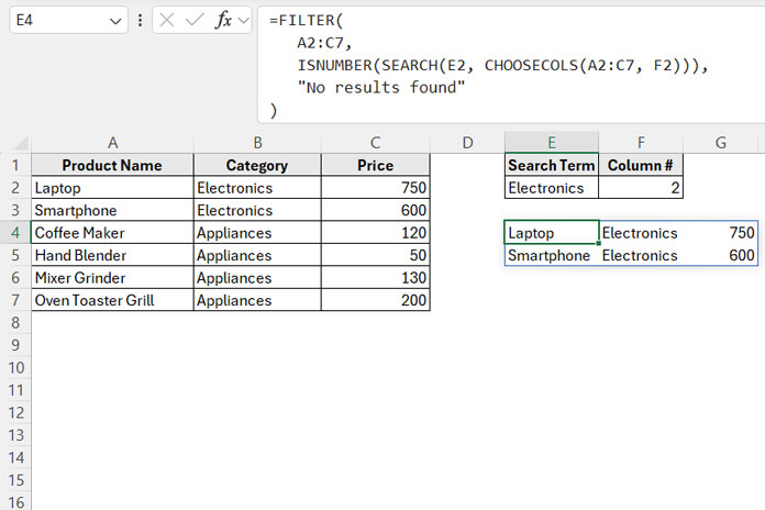
In cell E1, type Search Term, and in F1, type Column #.
Enter the search term (e.g., Electronics) in E2 and the column number (e.g., 2 for Category) in F2.
In E4, enter the following formula:
=FILTER(
   A2:C7,
   ISNUMBER(SEARCH(E2, CHOOSECOLS(A2:C7, F2))),
   "No results found"
)
Formula Explanation
FILTER Syntax:
FILTER(array, include, [if_empty])- array: The range to filter, in this case,
A2:C7. - include: The condition used to filter rows.
- if_empty: Custom message displayed when no results are found (e.g., “No results found!”).
Breaking Down the ‘include’ Argument:
ISNUMBER(SEARCH(E2, CHOOSECOLS(A2:C7, F2)))CHOOSECOLS(A2:C7, F2): Returns the column specified by the number in F2.- For example, entering
2in F2 selects the second column (Category).
- For example, entering
SEARCH(E2, …): Searches for the term in E2 within the selected column.- Returns a number if the search term is found; otherwise, it returns an error.
ISNUMBER(…): Converts the result of SEARCH into TRUE (if a match is found) or FALSE.- FILTER: Filters rows where the condition evaluates to TRUE.
What Happens If No Match Is Found?
If the search term is not found, the formula returns the custom message “No results found!”.
Searchable Table with FILTER: Entire Row
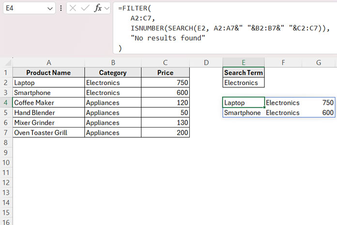
Instead of searching a specific column, you might want to search across all columns in each row. This is useful when you’re unsure where the search term might be located.
Here’s the formula to filter rows by searching the entire table:
=FILTER(
   A2:C7,
   ISNUMBER(SEARCH(E2, A2:A7&" "&B2:B7&" "&C2:C7)),
   "No results found"
)
Key Differences in This Formula
The ‘include’ argument concatenates all columns into a single text string for each row:
A2:A7 & " " & B2:B7 & " " & C2:C7- SEARCH checks for the search term (E2) across the combined row values.
- ISNUMBER returns TRUE for rows where the search term is found.
- FILTER extracts only the rows that match the search term.
For this approach:
- Omit F1 and F2 (no need to specify a column number).
- Enter the search term (e.g., “Electronics”) in E2.
That’s all about creating a searchable table with the FILTER function in Excel. Leave your feedback below, and feel free to suggest any additional improvements.
Resources for Further Learning
- Comparing the FILTER Function in Excel and Google Sheets
- Filter Data from the Previous Month Using a Formula in Excel
- Get Top N Values Using Excel’s FILTER Function
- Search Tables in Excel: Dynamic Filtering for Headers & Data
- Excel: Filter Data with a Dropdown and ‘All’ Option (Dynamic Array)
- How to Apply Nested Column and Row Filters in Excel
- Adding a Dynamic Total Row to Excel FILTER Function Results