To compare two tables with similar data for differences, you can use the XLOOKUP function in Excel. Drag the formula across as per the number of columns to check differences across each column. Then, use those values to highlight the differences.

If you want a dynamic formula, you can use the REDUCE lambda helper function to expand XLOOKUP dynamically.

In this tutorial, you will learn both methods for comparing two tables for differences in an Excel spreadsheet. Here are the prerequisites:

• The tables must contain a unique identifier column (e.g., product IDs, Employee IDs, etc.).
• The unique identifier must not be repeated in either table.
• The data can be in any order. The formula matches rows by their unique identifier, regardless of position.

Since the problem involves two tables, you can decide which table to highlight. Highlighting both tables is also possible. This tutorial will cover all scenarios.

Compare Table #1 with Table #2 for Differences

In the following examples, the sample tables are as follows:

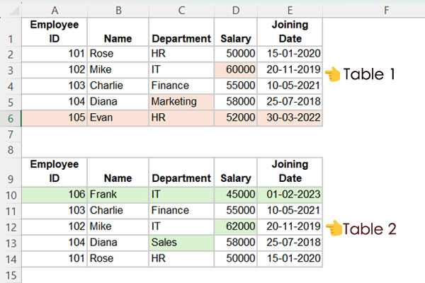
Employee IDs serve as the unique identifier in both tables.

Formula:

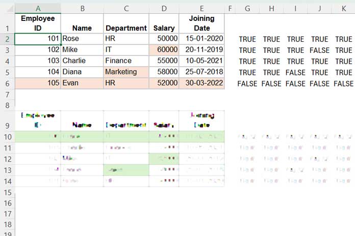
Enter the following formula in cell G2 and drag it across to column K to compare both tables and find the differences in Table #1:

=XLOOKUP($A$2:$A$6, $A$10:$A$14, A10:A14, "")=A2:A6

We will use the result to highlight the table range A2:E6.

Before proceeding, let’s quickly explain this formula.

Explanation:

• XLOOKUP searches the IDs in $A$2:$A$6 (Table #1) within the ID column $A$10:$A$14 (Table #2).
• If a match is found, it returns the corresponding value from column A10:A14.
• If no match is found, it returns an empty cell.
• The last part (=A2:A6) checks if the returned value matches the value in Table #1, outputting TRUE for matches and FALSE otherwise.

Steps to Highlight the Cells with Differences:

The TRUE or FALSE values generated by the formula act as a helper range to identify differences.

1. Select the range A2:E6 and go to Home > Conditional Formatting > New Rule.
2. In the New Formatting Rule dialog box, choose “Use a formula to determine which cells to format.”
3. Enter this formula:

=AND(A2<>"", NOT(G2))

4. Click Format and choose a style (e.g., a fill color).
5. Click OK to apply the formatting.

This will highlight cells in the first table that differ from or are missing in the second table.

Converting the Formula to a Dynamic Version

If you prefer not to drag the G2 formula across columns, use the following dynamic formula instead:

Formula:

=DROP(
   REDUCE(
      "", SEQUENCE(5), 
      LAMBDA(a, v, HSTACK(a, 
         XLOOKUP($A$2:$A$6, $A$10:$A$14, CHOOSECOLS(A10:E14, v), "")
      ))
   ), ,1
) = A2:E6

Formula Explanation

LAMBDA(a, v, HSTACK(a, XLOOKUP($A$2:$A$6, $A$10:$A$14, CHOOSECOLS(A10:E14, v), ""))) – This is the LAMBDA function that utilizes the XLOOKUP function.

If you compare the XLOOKUP function in this formula with the earlier drag-across one, you will notice that the result range A10:A14 in the previous formula has been replaced by CHOOSECOLS(A10:E14, v).

The REDUCE function iterates through each value in SEQUENCE(5), generating sequence numbers from 1 to 5. As a result, CHOOSECOLS(A10:E14, v) becomes CHOOSECOLS(A10:E14, 1), CHOOSECOLS(A10:E14, 2), …, up to CHOOSECOLS(A10:E14, 5).

Here, we compare the result with =A2:E6 since the formula returns the results as a whole array. In the drag-across formula, the comparison is made column-by-column, such as =A2:A6.

This method allows us to dynamically compare two tables for differences in Excel.

Compare Table #2 with Table #1 for Differences

Once you understand the previous steps, comparing Table #2 with Table #1 becomes straightforward. You only need to make minor adjustments to the formula and highlight rule.

Steps:

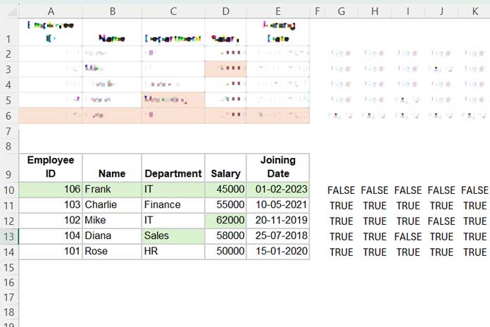
1. Enter the following formula in cell G10:

=XLOOKUP($A$10:$A$14, $A$2:$A$6, A2:A6, "")=A10:A14

2. Drag the formula across to column K.
3. To highlight differences in Table #2, use this formula in Conditional Formatting:

=AND(A10<>"", NOT(G10))

4. Apply this rule to the range A10:E14.

Dynamic Version:

=DROP(
   REDUCE(
      "", SEQUENCE(5), 
      LAMBDA(a, v, HSTACK(a, 
         XLOOKUP($A$10:$A$14, $A$2:$A$6, CHOOSECOLS(A2:E6, v), "")
      ))
   ),,1
)=A10:E14

This approach is analogous to the dynamic formula for Table #1 and can dynamically compare the entirety of Table #2.

Conclusion

We explored both dynamic and non-dynamic approaches to compare two tables for differences in Excel. You can stick with the non-dynamic formula if you’re not comfortable with advanced functions like LAMBDA. However, using the dynamic formula makes the process more efficient, especially for larger tables.

Remember:

• Modify range references to fit your data.
• Replace the number 5 in SEQUENCE with the actual number of columns in your tables.

Additional Resources:

• Comparing Two Sets of Multi-Column Data for Differences in Google Sheets
• Combine Two Tables in Excel Using a Dynamic Array Formula
• Flip a Table Vertically in Excel (Includes Dynamic Array Formula)
• Search Tables in Excel: Dynamic Filtering for Headers & Data
• How to Create a Searchable Table in Excel Using the FILTER Function