")


")


")

")
")
 in Excel & Google Sheets")


We may not always need to perform a case-sensitive XLOOKUP for product names in Excel. However, when dealing with product codes, case sensitivity can be crucial. For instance, an item code AL1145a and AL1145A might represent the same product but in different quality grades.
By default, lookup functions in Excel are case-insensitive. To make them case-sensitive, we need a workaround. This tutorial explains how to perform a case-sensitive XLOOKUP in Excel by combining the EXACT function with XLOOKUP.
Example: Case-Sensitive XLOOKUP in Excel
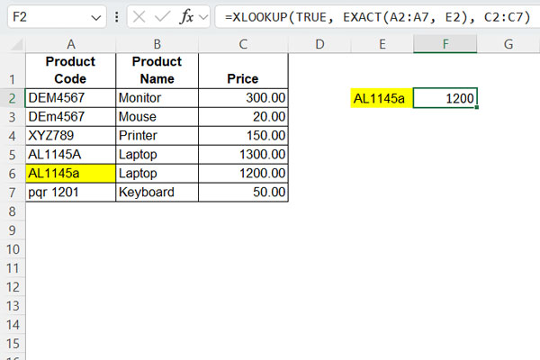
Consider a dataset where:
- Product codes are in A2:A7,
- Product names are in B2:B7, and
- Prices are in C2:C7.
You want to look up a product code entered in E2 and return its price. Since product codes are case-sensitive, you need a case-sensitive XLOOKUP. Use the formula below:
=XLOOKUP(TRUE, EXACT(A2:A7, E2), C2:C7)This formula ensures you retrieve the price for the exact match based on case.
Returning Both Product Name and Price
To return both the product name and price, replace the result range C2:C7 with B2:C7 in the formula:
=XLOOKUP(TRUE, EXACT(A2:A7, E2), B2:C7)Formula Explanation
In this formula, the components are as follows:
- Lookup Value:
TRUE - Search Range:
EXACT(A2:A7, E2) - Result Range:
B2:C7
How it Works:
- The EXACT function compares the product code in E2 with each code in A2:A7, returning TRUE for exact case-sensitive matches and FALSE otherwise.
{FALSE;FALSE;FALSE;FALSE;TRUE;FALSE} - XLOOKUP uses
TRUEas the lookup value to locate the exact match in the array of TRUE/FALSE values returned by EXACT. - The corresponding value from B2:C7 is returned as the result.
Can I Use Multiple Search Keys in a Case-Sensitive XLOOKUP?
In a standard XLOOKUP, you can look up multiple search keys (lookup values). For example:
=XLOOKUP(E2:E3, A2:A7, C2:C7)Where E2:E3 contains the lookup values.
However, with a case-sensitive XLOOKUP in Excel, this isn’t directly possible because the search range depends on the TRUE/FALSE array from EXACT. To handle multiple search keys, you need to combine the formula with a custom LAMBDA function and use the MAP function.
Handling Multiple Lookup Values with LAMBDA and MAP
Step 1: Convert XLOOKUP-EXACT Combo to a LAMBDA Function
The original formula:
=XLOOKUP(TRUE, EXACT(A2:A7, E2), C2:C7)is converted into a LAMBDA function as follows:
LAMBDA(val, XLOOKUP(TRUE, EXACT(A2:A7, val), C2:C7))Here, val is defined within the LAMBDA function for dynamic lookup.
Step 2: Use MAP to Apply LAMBDA Across Multiple Keys
Use the MAP function to iterate through multiple keys in E2:E3:
=MAP(E2:E3, LAMBDA(val, XLOOKUP(TRUE, EXACT(A2:A7, val), C2:C7)))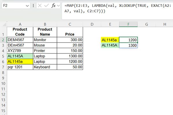
The MAP function applies the LAMBDA formula to each value in E2:E3, performing case-sensitive lookups for each lookup value.
Conclusion
By combining EXACT with XLOOKUP, and using LAMBDA and MAP, Excel enables precise case-sensitive lookups for both single and multiple keys. This method is flexible and powerful, ensuring data accuracy in scenarios where case sensitivity is critical.