


The FVSCHEDULE function in Google Sheets is simple to learn if you know the use of the FV function.
Unlike in FV where a fixed interest rate is applied, in the FVSCHEDULE function, we can specify a series of potentially varying interest rates as an array.
The purpose of the FVSCHEDULE function is to return the future value aka FV of the initial principal payment (PV) based on a series of compounding interest rates.
Compounding interest rates are calculated based on both the initial principal and the accumulated interest from previous periods. In the formula, you just need to specify the rates as an array.
The FVSCHEDULE function in Google Sheets is useful in investment decision making.
For example, assume an investment guarantees a certain (let us say 4%) percentage for the first year, 5% in the second year, and 6% in the third year. If so, we can evaluate this investment using the FVSCHEDULE function.
You can learn more about this financial function usage after the Syntax part below.
Syntax of the FVSCHEDULE Function in Google Sheets
Syntax:
FVSCHEDULE(principal, rate_schedule)Arguments:
principal – The amount of initial capital or value to compound against (Present Value aka PV).
rate_schedule – An array/range of interest rates to compound against the principal.
I will explain more about how to specify the rate_schedule in the FVSCHEDULE function in Google Sheets with an example below.
Example to the Use of the FVSCHEDULE Function in Google Sheets
Suppose I invest $ 10,000 that will return 4% in the first year, 3.5% in the second year, and 3% in the third year.
Let us use the FVSCHEDULE function to calculate the future value of this particular investment.
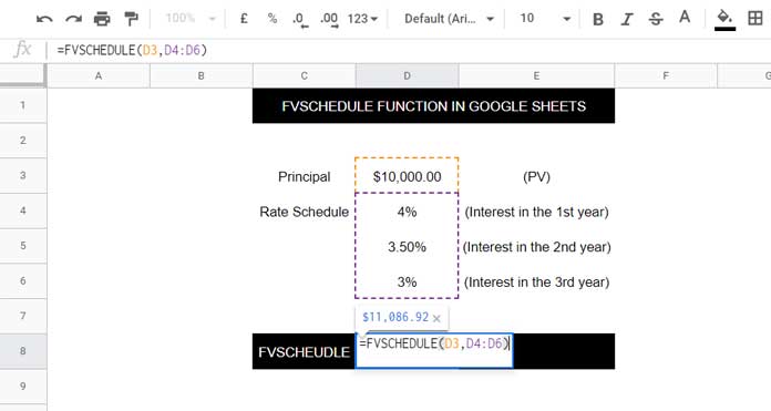
In the above formula the PV is in cell D3 and the varying interest rates are in the range D4:D6.
As you can see, the formula returns $11,086.92.
Usage Notes:
You can specify the rate_schedule three ways in the formula. They are as follows.
- In a percentage format (in D4:D6) as per the above formula example.
- Numbers within UNARY_PERCENT as;
- The formula to be used in D4
=UNARY_PERCENT(4) - in D5
=UNARY_PERCENT(3.5) - In D6
=UNARY_PERCENT(3)
- The formula to be used in D4
- Decimals like 0.04, 0.035, and 0.03 in D4, D5, and D6 respectively.
If you hardcode the above values, i.e. the PV and the Interest Schedule within the FVSCEDULE function in Google Sheets, the formula would be as follows.
=FVSCHEDULE(10000,{0.04,0.035,0.03})The formula treats, blank cells, if any, in the cells as 0. No doubt, the formula would return #VALUE! error incase any text/string (non-numeric values) present in the cells.
Fixed Interest Rates in the Interest Schedule
This section is meant to help you understand the difference between the FV and FVSCHEDULE functions in Google Sheets.
Here are two examples. One using the FV and the other using the FVSCHEDULE.
Here are my two formulas.
In cell D8;
=FVSCHEDULE(D3,D4:D6)See the interest rate is 4% in all the three years (please refer to the below image).
The above formula would return $11,248.64.
In cell H8;
=FV(H3,H4,H5,H6)This formula would also return the same result.
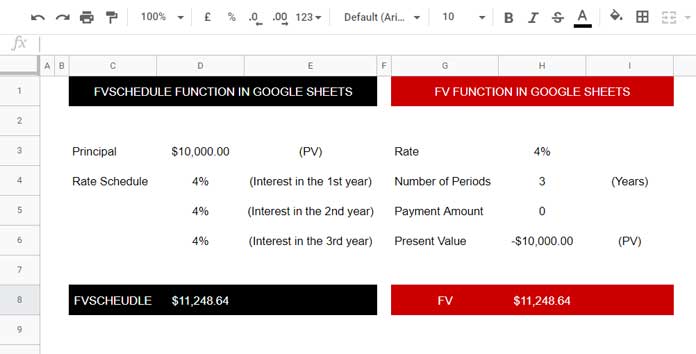
What I am trying to say is if the interest rate is fixed, then use the FV function whereas if the interest rates are varying, then use the FVSCHEDULE function.
That’s all. Enjoy!