


In this post, get the formula to properly convert seconds to HH:MM:SS format in Google Sheets.
For example, the elapsed time is 100,000 seconds in cell C2. My formula in cell D2 will convert this elapsed time in seconds to 1 day 03:46:40.
How?
Some of you may think that by formatting cell C2 or using a TEXT function in cell D2 (given after a few paragraphs below), you can achieve the above result. It won’t work on the contrary!
For example, cell C2 contains the elapsed time in seconds (100,000) that you want to convert to hours, minutes, and seconds in HH:MM:SS time format in Google Sheets.
Select this cell (just click C2) and apply Format (menu) > Number > Duration or Format (menu) > Number > Time. Both will give you wrong results.
Even the following Text formula wont convert the total seconds to the said time format!
=text(C2,"HH:MM:SS")Then what is the solution?
In any cell, for example, cell D2, if you divide C2 by 86,400 (60 seconds * 60 minutes * 24 hours = 86,400), then you can format that cell to the duration from the format menu.
You will get the correct duration as below.
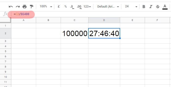
Instead of Duration, if you select Time format, then you will get 03:46:40. It skips 24 hours (day), so obviously not correct, anyway, right?
Get the correct solution, which is a formula, step-by-step below.
Convert Seconds to HH:MM:SS, but Not to Duration, in Google Sheets
If you want to convert seconds to time format like HH:MM:SS as below in Google Sheets, then please read on.
I’ll use four simple functions as a combination. Those functions are TRUNC, MOD, TEXT, and IFS.
I’ll guide you on how to combine these functions based formulas and create seconds to HH:MM:SS converter in Google Sheets.
Refer: Google Sheets Function Guide.
First, we will apply two key formulas (TRUNC and MOD+TEXT) in cell D5 and D6. We can remove these formulas later.
Here are the steps, one by one.
Steps
Step 1: TRUNC formula in cell D5 that returns the number of days from the total seconds in cell C2.
=trunc(C2/86400)Step 2: MOD + TEXT formula in cell D6 that returns the remaining seconds in time format.
That means the balance seconds in time format after converting the total seconds in cell C2 to days in the above step # 1.
=text(mod(C2/86400,1),"HH:MM:SS")Step 3: In cell D2, just combine these two formulas and place the text “days” in between. Also, if you want, you can now empty the cells D5 and D6 (I suggest keep it for later use/reference).
=trunc(C2/86400)&" days "&text(mod(C2/86400,1),"HH:MM:SS")We have created a formula that converts seconds to HH:MM:SS time format in Google Sheets.
But this combination has two visible issues! What’s that?
Assume the total elapsed seconds that we want to convert to the format day, hours, minutes, and seconds in Google Sheets is only 60 seconds. The above formula would convert 60 seconds to 0 days 00:01:00 instead of just 00:01:00.
In another scenario, if the seconds to convert are 150000, then the result would be 1 days 17:40:00 instead of 1 day 17:40:00.
That means we should clean the output someway. For that, we can use either of the IF or IFS logical functions. I’m proceeding with the IFS function.
How?
We just want to check whether the number of days underlying in the total elapsed seconds is less than or equal to zero, one, or greater than one.
The formula that returns the number of days underlying in the total elapsed seconds is the TRUNC formula in cell D5. We can use IFS to test it, i.e. <=0, =1, or >1.
=ifs(
     trunc(C2/86400)<=0,,
     trunc(C2/86400)=1,
        trunc(C2/86400)&" day",
     trunc(C2/86400)>1,
        trunc(C2/86400)&" days")&" "&text(mod(C2/86400,1),"HH:MM:SS"
)
The above is our final formula in cell D2 to convert seconds to HH:MM:SS format in Google Sheets. Please find the sample sheet below.
Thanks for the stay, enjoy!