


In your leisure, try to learn all the essential and popular financial functions in Google Sheets. It’ll help you to take bold financial decisions in your personal/official life. The PV function in Google Sheets one such essential function to learn.
Try to learn at least one Financial spreadsheet function. So you will realize that it’s easy to learn other functions in this category too. If you ask me which function, to begin with, no doubt I will recommend the PMT function.
In this Spreadsheet tutorial, I am going to explain how to use the PV function in Google Sheets. PV is the short form of Present Value.
The purpose of the PV function in Google Sheets is to calculate the present value of a loan/investment based on a constant periodic payment and interest rate. In concise PV is the present value of money that you will get in the future.
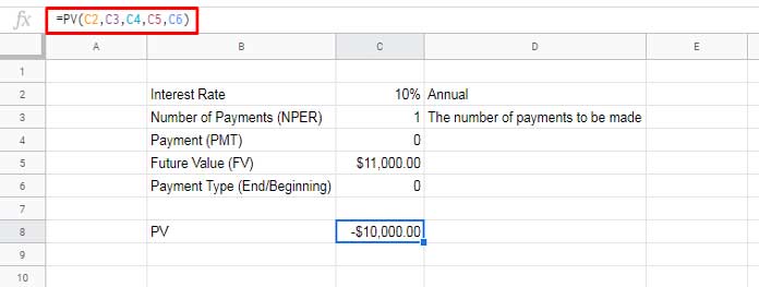
As an example, with a 10% annual interest rate and annual payment, the present value (PV) of $11,000 a year from now will be $10,000. In this $11,000 is Future Value and $10,000 is its Present Value.
I will explain this in the PV function formula example part. Right now, please take the time to understand the syntax part.
The Syntax of the PV Function in Google Sheets
PV(rate, number_of_periods, payment_amount, [future_value], [end_or_beginning])Function Arguments:
rate – The annual interest rate. Based on the period monthly/quarterly/yearly, you may need to divide the interest rate by 12 (monthly) and 4 (quarterly).
number_of_periods (Nper) – The number of payments to be made. If the tenure of a loan is 5 years and you make monthly payments, you must enter Nper as 60 (5*12).
payment_amount (Pmt) – The payment to be made in each period. If Pmt is omitted, don’t forget to include the future value (FV).
future_value (FV) – A cash balance remaining after the last payment is made. That means your investment goal. It’s optional.
end_or_beginning – The number 0 or 1 and indicates whether the payments are due at the end or at the beginning.
Formula Examples to Google Sheets PV Function
In the beginning, I have given you one example. Here is that formula part.
Assume you will get a loan to the tune of $11,000.00 next year (FV) and the interest rate is 10%. The Present Value (PV) of that amount will be $10,000.00.
We can use the PV function in Google Sheets to calculate that Present Value very easily.
See the inputs like annual interest rate (10%), number of periods (1 year), and FV in the screenshot. That can help you to understand the formula.
PV Formula in Monthly/Quarterly/Yearly Payments
In the above PV function example, I have considered a lump-sum payment (FV) to calculate the PV. But in the coming examples, let me use the PV function to calculate the PV of periodic payments for a period of 5 years.
The PV function output will be slightly different based on the payment terms. I mean you will get different PV for monthly payments, quarterly payments, and as well as in yearly payments.
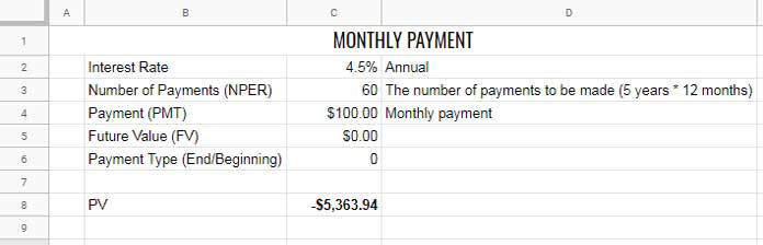
Monthly:
The formula is in cell C8 (sorry that I missed that in the screenshot).
=PV(C2/12,C3,C4,C5,C6)Since the payment mode is monthly, you must divide the annual interest rate by 12.
Quarterly:
When you calculate PV in quarterly payments, the input values and formula will be slightly different.
Here instead of dividing the interest rate by 12, divide it by 4 (quarterly).
=PV(C2/4,C3,C4,C5,C6)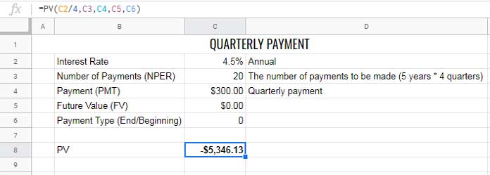
In this PV formula, the NPER is 20. That means the total number of payments in 5 years will be 20 (5 * 4). Also, as mentioned above, the annual interest rate must be divided by 4 to make its quarterly interest rate.
Yearly:
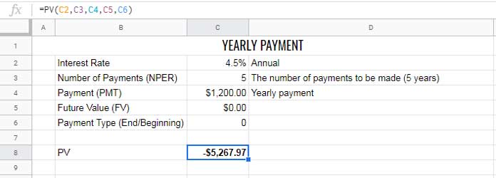
=PV(C2,C3,C4,C5,C6)Here use the interest rate as it is.
Conclusion
Hope I have well explained the topic of how to use the PV function in Google Sheets. I think a comparison of the financial function FV and PV is required. It’s in the pipeline and I will update you about that soon!
For more Financial function tutorials, please check my Google Sheets function guide.