We can use a combination of XLOOKUP and VLOOKUP in both Excel and Google Sheets to look up values under categories. If the formula returns a result from a single column, the formula remains the same. However, if multiple columns are involved, the only change is the application of the ARRAYFORMULA in Google Sheets.
In spreadsheets, we often don’t follow strict database-like rules for entering data. Spreadsheets are versatile tools that allow us to manage both structured and unstructured data. A common example of unstructured data is when multiple categories and subcategories are stored in the same column. This structure can make it challenging to look up specific values under specific categories.
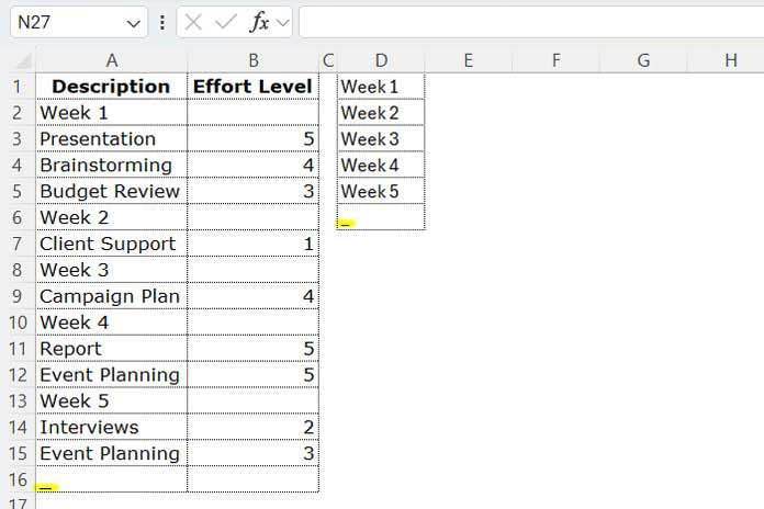
For example, consider the following dataset in A1:B15:
| Description | Effort Level |
| Week 1 | |
| Presentation | 5 |
| Brainstorming | 4 |
| Budget Review | 3 |
| Week 2 | |
| Client Support | 1 |
| Week 3 | |
| Campaign Plan | 4 |
| Week 4 | |
| Report | 5 |
| Event Planning | 5 |
| Week 5 | |
| Interviews | 2 |
| Event Planning | 3 |
How do you look up the task “Event Planning” under the category “Week 4” when it also appears under the category “Week 5”?
In this tutorial, we’ll explore how to look up values under specific categories in Excel and Google Sheets.
Lookup Values Under Categories in Excel
Follow these step-by-step instructions to solve the problem in Excel:
Steps:
- Define the Categories:
Enter the categories (e.g., “Week 1” to “Week 5”) in D1:D5. - Mark the End of the Data:
Enter an underscore (_) in A16 to indicate that the dataset ends in the previous row. - Mark the End of the Categories:
Enter an underscore (_) in D6 to indicate that the category list ends.
- Enter Lookup Values:
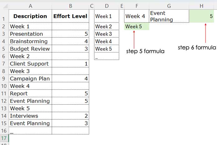
- Specify the category to look up (e.g., “Week 4”) in F1.
- Enter the value to search for under the specified category (e.g., “Event Planning”) in G1.
- Extract the Next Category:
In F2, use the following helper formula to extract the next category:=OFFSET(XLOOKUP(F1, D1:D6, D1:D6), 1, 0) - Look Up the Value:
In H1, use this formula to look up the value specified in G1 under the category specified in F1:
=VLOOKUP(G1, XLOOKUP(F1,A2:A16,A2:A16):XLOOKUP(F2,A2:A16,B2:B16), 2, 0)
Anatomy of the Formula:
XLOOKUP(F1, A2:A16, A2:A16):
Finds the first occurrence of the category specified in F1 (e.g., “Week 4”).
The lookup range isA2:A16, and the result range is alsoA2:A16, which allows it to return the row where the specified category is found.XLOOKUP(F2, A2:A16, B2:B16):
Finds the start of the next category specified in F2.
The lookup range isA2:A16(same as the first XLOOKUP), but the result range isB2:B16(the Effort Level column), which allows it to return the corresponding Effort Level for the next category.- The Range:
By combining these twoXLOOKUPfunctions with a colon (:), we create a dynamic range between the category specified in F1 and the next category specified in F2. This dynamic range is then used by the VLOOKUP function to search within the correct section of the data.
| Week 4 | 0 |
| Report | 5 |
| Event Planning | 5 |
| Week 5 | 0 |
VLOOKUP(G1, ..., 2, 0):
This part of the formula searches for the value in G1 (e.g., “Event Planning”) within the defined range and returns the corresponding Effort Level from column B (the second column of the range). The2in the formula specifies the second column, and0ensures an exact match.
This formula locates the search key “Event Planning” under the specified category (e.g., “Week 4”) and returns the Effort Level from the corresponding row in column B.
Lookup Values Under Categories in Google Sheets
The process in Google Sheets is nearly identical to Excel. You can use the same steps and formulas to look up values under specific categories.
Handling Multiple Columns
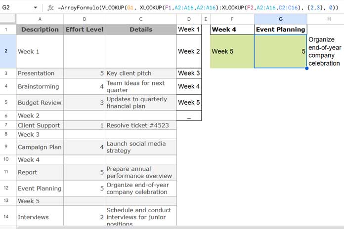
If your table has an additional column (e.g., Details in C1:C16) and you want to return values from both the “Effort Level” and “Details” columns, adjust the formula:
Excel Formula:
=VLOOKUP(G1, XLOOKUP(F1, A2:A16, A2:A16):XLOOKUP(F2, A2:A16, C2:C16), {2, 3}, 0)Google Sheets Formula:
In Google Sheets, wrap the formula with ARRAYFORMULA to handle arrays:
=ArrayFormula(VLOOKUP(G1, XLOOKUP(F1, A2:A16, A2:A16):XLOOKUP(F2, A2:A16, C2:C16), {2, 3}, 0))Here:
- The second XLOOKUP now references
C2:C16, and the VLOOKUP includes an array constant{2,3}to return multiple columns.

Summary
This tutorial shows how to use Excel and Google Sheets to look up values under specific categories in a dataset. By combining XLOOKUP and VLOOKUP, we can isolate and search within dynamically defined ranges.


