The UMINUS function in Google Sheets is an operator function that reverses the sign of a number. Without using this function, you can still reverse the sign of a number in Google Sheets by multiplying the number by -1.
UMINUS Equivalent: If you multiply a number by -1, the sign of that number will be reversed.
For example, in the formula =A1*-1 in cell B1, the sign of the value in cell A1 will be reversed.
UMINUS Function Examples in Google Sheets
UMINUS Function: Syntax and Argument
Syntax:
=UMINUS(value)
- value: The specific number whose sign you want to reverse.
Note:
The UMINUS function will return #VALUE! if the value is text. If the value is a number or a percentage, it will reverse the sign. Additionally, applying the function to a date or time will produce an unintended result.
Examples of the UMINUS Function in Google Sheets
Let’s say cell A1 contains the value 54. The following formula in cell B1 would return -54:
=UMINUS(A1)When you have a list of numbers whose signs you want to reverse, you can use the UMINUS function in an array formula. For example, to reverse the sign of numbers in the range A1:A, you can use the following formula in cell B1:
=ARRAYFORMULA(UMINUS(A1:A))Using UMINUS with IF Function
Assume you have a table with the following data:
| Description | Dr/Cr | Amount |
| Salary | Cr | 2,500.00 |
| Grocery Expense | Dr | 200.00 |
| Rent Expense | Dr | 1,200.00 |
| Freelance Income | Cr | 800 |
| Freelance Income | Cr | 800.00 |
| Dividend Income | Cr | 300 |
| Profit on Sale of Assets | Cr | 1,000 |
| Utility Bills | Dr | 150.00 |
| FD Interest | Cr | 150 |
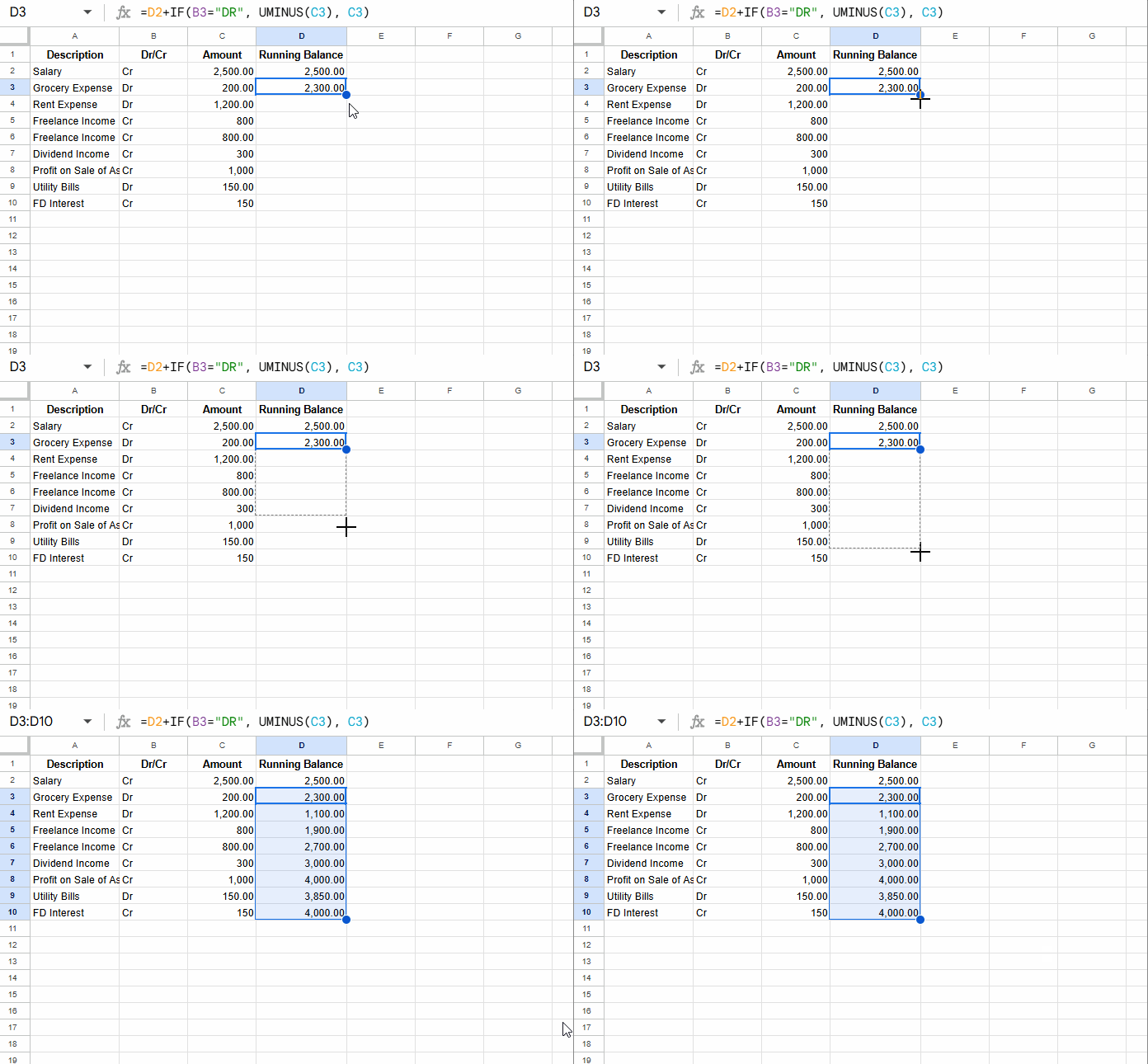
To calculate the running balance, you can use the UMINUS function in Google Sheets with an IF statement. Here’s how to do it:
- In cell D2, enter
=C2. - In cell D3, enter the formula:
=D2 + IF(B3="DR", UMINUS(C3), C3)and drag the fill handle of D3 down to apply the formula to the rest of the column.

This formula will reverse the sign of the amount if the value in the “Dr/Cr” column is “Dr”. If the value is “Cr”, the amount will remain unchanged.
Alternatively, you can use this array formula in cell D2:
=SCAN(0, C2:C10, LAMBDA(acc, val, acc + IF(OFFSET(val, 0, -1)="dr", UMINUS(val), val)))Additional Tip: Using the UPLUS Function
The UPLUS function returns the input number unchanged! This function exists in Google Sheets for compatibility with other spreadsheet applications.
Here is the syntax of the UPLUS function:
=UPLUS(value)For example, if the value in cell A1 is 50, the formula =UPLUS(A1) would return 50. If the value in A1 is -50, the formula will return -50.
While the UPLUS function is available, it’s generally not necessary to use it unless you’re working in a multi-platform environment where compatibility is required.


