The TREND function in Google Sheets is an excellent tool for simple forecasting. It returns values along a linear trend using the least squares method. With the TREND function, you can predict future data points, such as demands, based on existing trends.
As a side note, the TREND function is an array formula that can return multiple results in a range without the need to use the ARRAYFORMULA function.
TREND Function: Syntax and Basic Example
Syntax:
TREND(known_data_y, [known_data_x], [new_data_x], [b])Let me explain the arguments using formula examples.
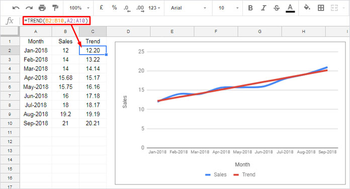
Below is an example of the TREND function in Google Sheets. It calculates a trend line based on sales data over 9 months (from January to September) using the formula:
=TREND(B2:B10, A2:A10)
The accompanying chart shows a straight trendline, which illustrates the linear relationship of sales over time.
This trendline is created using the least squares method, as applied by the TREND function with the formula =TREND(B2:B10, A2:A10).
The method fits a straight line to your existing data points in B2:B10 (sales data) and A2:A10 (corresponding months). It minimizes the sum of the squared differences between the actual data points and the values on the trend line, providing the best fit for the given data.
To make predictions, you need to include new x-values (new_data_x) in the formula. In the above TREND formula (see cell C2 in the image), I’ve used only part of the arguments. What are they?
TREND(known_data_y, [known_data_x])Here are the details:
known_data_y: This range, B2:B10, contains the known dependent (y) values (sales data) used to fit an ideal linear trend.known_data_x: These are the values of the independent variable (the months in the range A2:A10) that correspond to theknown_data_y.
I’ll explain the remaining function arguments with the example below.
Analyzing Sales Over Time and Predicting Future Demand with the TREND Function
In the above TREND function example, I have sales data from January to September, and I want to forecast sales for the upcoming months. Let’s see how to do that in Google Sheets using the TREND function.
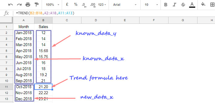
I want to predict sales for the months of October through December. The following formula in cell B11 will return the forecasted sales for those months:
=TREND(B2:B10, A2:A10, A11:A13)
Where:
known_data_y: B2:B10 (the sales data for January to September)known_data_x: A2:A10 (the corresponding months)new_data_x: A11:A13 (the months for which we want to forecast sales)
In this example, I haven’t specified the last argument, which is b, so the default value is assumed, i.e., TRUE.
What does this mean?
When b is omitted or set to TRUE, the formula calculates the trend line with a y-intercept that best fits the data. If b is set to FALSE, the trend line is forced to start from the point where the x-axis and y-axis meet (the origin).
Here’s a table illustrating the effect of specifying b in the TREND function:
| Month | Actual Sales | Forecasted Sales (b=TRUE) | Forecasted Sales (b omitted) |
| 1/1/2018 | 11 | ||
| 1/2/2018 | 22 | ||
| 1/3/2018 | 33 | ||
| 1/4/2018 | 44 | ||
| 1/5/2018 | 55 | ||
| 1/6/2018 | 66 | ||
| 1/7/2018 | 77 | ||
| 1/8/2018 | 88 | ||
| 1/9/2018 | 99 | ||
| 1/10/2018 | 55.25 | 110.20 | |
| 1/11/2018 | 55.28 | 121.44 | |
| 1/12/2018 | 55.32 | 132.32 |
Resources
Here are some related tutorials for Google Sheets.


This was really helpful!
Can you please also share when it’s wise to use this formula vs Growth formula?
I tried using the Growth formula but, it did not work in some cases because certain values were at 0.