Top N Products and Top N Sellers in Google Sheets (Top N of Top N)

If you’ve ever wanted to compare which sellers contribute the most to your top-selling products, this tutorial is for you. In this guide, I’ll show you how to dynamically generate a clean, chart-friendly summary table in Google Sheets that highlights:

The top N products based on total quantity sold
For each product, the top N sellers by quantity
In a layout perfect for column or bar charts

All with a single dynamic array formula. No helper columns. No scripts.

You’ll also learn how the formula smartly handles ties and why the layout is ideal for dashboards.

What We’re Building

Assume you want to find your top 3 selling products and the top 3 sellers for each of these products. Here’s the final output—a dynamic summary table that updates automatically as your data changes:

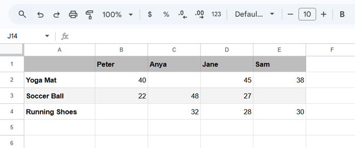
Top N Products and Top N Sellers summary table in Google Sheets with products as rows, sellers as columns, and quantities as values

You can plug this table directly into a chart. Want to visualize how each seller performs across your top products? Done. Need a quick snapshot of your salesforce’s impact? No problem.

The Sample Data

Here’s a preview of the raw data from columns A to C in Sheet1:

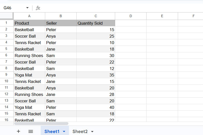
Raw sample data in Google Sheets showing Product, Seller, and Quantity Sold columns used to calculate top products and sellers

You’ll notice multiple rows for the same product-seller combination — that’s perfectly fine. The formula will automatically summarize them correctly.

To follow along, make a copy of my sample sheet here.

The Formula to Return Top N Products and Top N Sellers in Google Sheets

Paste the following formula into an empty cell in Google Sheets. Since it outputs a full table, it’s best to use cell A1 of a blank sheet within the same workbook that contains your data.

=ArrayFormula(LET(n_product, 3, n_seller, 3, data, Sheet1!A2:C,
   product_summary, 
      QUERY(data, "select Col1, sum(Col3) where Col1 is not null group by Col1 label sum(Col3)''", 0), 
   top_products, 
      CHOOSECOLS(SORTN(product_summary, n_product, 1, 2, 0), 1), 
   unique_sellers, 
      TOROW(UNIQUE(CHOOSECOLS(data, 2)), 3), 
   top_sellers, 
      MAP(top_products, LAMBDA(val, VLOOKUP(unique_sellers, SORTN(QUERY(FILTER({CHOOSECOLS(data, 2), CHOOSECOLS(data, 3)}, CHOOSECOLS(data, 1)=val), "select Col1, sum(Col2) group by Col1 label sum(Col2)''", 0), n_seller, 1, 2, 0), 2, 0))), 
   fnl, 
      IFNA(VSTACK(HSTACK(, unique_sellers), HSTACK(top_products, top_sellers))), 
   fnl
))

This formula returns a Top N of Top N summary in Google Sheets—meaning:

Top 3 products based on total quantity sold.
For each product, the top 3 sellers based on their respective quantity sold.

You can easily customize this:

Change 3 (used in n_product) to set how many top products you want.
Change 3 (used in n_seller) to set how many top sellers you want for each product.

Adjust the Data Range if Needed

If your source data isn’t in Sheet1!A2:C, update this part accordingly:

Replace Sheet1!A2:C with the actual range containing your data.
If your data includes more than three columns, you’ll need to construct a 3-column array like this: HSTACK(Sheet1!A2:A, Sheet1!B2:B, Sheet1!C2:C)

This formula dynamically calculates and returns a chart-ready summary of the top N products and their top N sellers in Google Sheets, with no scripts or helper columns required.

How It Works (Step-by-Step)

Step 1: Set the N values

n_product, 3,
n_seller, 3,

These values control how many top products and top sellers per product the formula will return.

For example, if you update them to:

n_product, 5,
n_seller, 3,

The output will include the top 5 products based on quantity sold, and for each of those products, the top 3 sellers.

Step 2: Get total quantity per product

product_summary, 
      QUERY(data, "select Col1, sum(Col3) where Col1 is not null group by Col1 label sum(Col3)''", 0),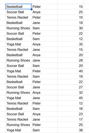

Google Sheets QUERY function summarizing total quantity sold for each product to identify top-selling items

Step 3: Get the top N products

top_products, 
      CHOOSECOLS(SORTN(product_summary, n_product, 1, 2, 0), 1),

Handling ties:

If two or more products are tied at the nth position, SORTN includes all of them, so your results may include more than n products in such cases.

Step 4: List all unique sellers

unique_sellers, 
      TOROW(UNIQUE(CHOOSECOLS(data, 2)), 3),

This flattens the sellers horizontally to form the header row.

Step 5: For each top product, get top N sellers

top_sellers, 
      MAP(top_products, LAMBDA(val, VLOOKUP(unique_sellers, SORTN(QUERY(FILTER({CHOOSECOLS(data, 2), CHOOSECOLS(data, 3)}, CHOOSECOLS(data, 1)=val), "select Col1, sum(Col2) group by Col1 label sum(Col2)''", 0), n_seller, 1, 2, 0), 2, 0))),

This part loops through each top product (top_products) and returns its top n_seller sellers based on total quantity sold.

Handling ties:

Just like before, SORTN includes all sellers tied at the nth position, so the actual number of sellers may exceed n if there’s a tie.

Step 6: Stack the table neatly

fnl, 
      IFNA(VSTACK(HSTACK(, unique_sellers), HSTACK(top_products, top_sellers))),

This combines the pieces into a tidy table, with seller names in the header row and product names in the first column.

Why This Format Is Ideal for Charts

You could try to build a Pivot Table with a similar structure, but it would include all products and sellers. Since you’re only interested in the top N products and top N sellers for each product, this formula-based solution is much more streamlined and dashboard-ready.

This layout is perfect for:

Column charts (one per product)
Stacked bar or column charts to compare sellers
Sparklines inside cells (as a compact visual summary)

Optional Bonus: Add Sparklines in the Last Column

To insert sparklines, paste the following formula into cell F2 (assuming your result table spans columns A to E), then drag down:

=SPARKLINE(B2:E2, {
  "charttype", "column";
  "color", "#bdcf32";
  "lowcolor", "#ea5545";
  "highcolor", "#50e991";
  "empty", "ignore"
})

This creates a mini column chart in each row.

Full-Scale Chart Instead?

If you’d prefer a full-size chart instead of sparklines:

Select the result table (e.g., A1:E4)
Go to Insert > Chart
Choose Stacked Column Chart as the Chart Type
Uncheck “Switch rows/columns” if it’s selected

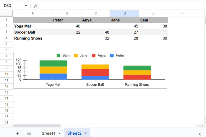
Stacked bar chart in Google Sheets visualizing top N sellers for top N products using chart-ready formula output

You now have a clean, insightful Top N Products and Top N Sellers chart ready for your Google Sheets dashboard.

Make It Dynamic (Optional Tip)

You can link n_product and n_seller to two input cells:

n_product, A1,
n_seller, B1,

Now users can change the table size without editing the formula.

Frequently Asked Questions (FAQ)

1. How can I get the top-selling products in Google Sheets?

To get the top-selling products in Google Sheets, you can use either a Pivot Table or a formula-based approach. For dynamic and customizable results, formulas are often more flexible.

Here are two helpful tutorials:

2. What is the best way to find top sellers for each product in Google Sheets?

You can find top sellers for each product by using the VLOOKUP function in combination with SORTN and QUERY. This formula allows you to identify the sellers who sold the most of each product. Our formula in this tutorial shows you how to get the top N sellers for each product.

3. How does the formula handle ties when multiple products or sellers have the same rank?

The formula uses the SORTN function, which can handle ties by ranking products or sellers based on quantity sold. It ensures that if there’s a tie at the nth position, the formula includes all tied entries, preserving the correct top N rank.

4. Can I adjust the formula to show more than the top 3 products or sellers?

Yes! The formula in this tutorial is adjustable. You can change the values for n_product and n_seller to show more products or sellers in your results. For example, changing n_product from 3 to 5 will display the top 5 products.

5. How do I use this formula in Google Sheets for different data sets?

To use this formula with your own data, simply replace the sheet names and ranges (e.g., Sheet1!A2:C) with the relevant references for your dataset. The structure remains the same, and the formula will work dynamically with your data.

Wrapping Up

With one formula, you now have a powerful way to report on:

Your best products
Your most effective sellers per product
All in a format perfect for charts