There are three main ways to convert a numeric value to a text value: using the TO_TEXT function, combining it with an empty string, or applying text formatting.
The importance of the TO_TEXT function lies in its ability to retain the original formatting of a numeric value. For example, a date will remain a date (not just a date value), and a currency-formatted number will keep its currency formatting, along with other value formats.
In contrast, the other two methods are less reliable. Combining with an empty string removes the original formatting, while text formatting retains it in most cases but loses the formatting if the value is the output of a formula.
In some cases, especially with mixed data types, the TO_TEXT function can be particularly useful. For instance, you may want to use it with QUERY to sort out mixed data types in a column.
Let’s start with the basic use of the TO_TEXT function and then move on to the QUERY example.
TO_TEXT Function: Syntax and Formula Examples
Syntax:
TO_TEXT(value)- where ‘value’ is the value to convert to text format.
Examples:
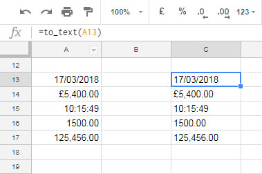
In the following example, cells A13:A17 contain different types of values, such as dates, currency-formatted numbers, time, etc.
Drag the following formula in cell C13 down to C17:
=TO_TEXT(A13)
If you want to convert all the values in the range A13:A17 to text format at once, you can use the TO_TEXT function as an array formula:
=ArrayFormula(TO_TEXT(A13:A17))Using the TO_TEXT Function in Google Sheets QUERY
Assume you have the following data in columns A1:B in Google Sheets:
| ID | Area |
| 123 | NORTH |
| 456 | NORTH |
| John | NORTH |
| 789 | SOUTH |
| Alice | NORTH |
You may try the following QUERY formula to filter the table where the second column matches “NORTH”:
=QUERY(A1:B, "SELECT * WHERE Col2='NORTH'", 1)However, the formula will return the following output:
| ID | Area |
| 123 | NORTH |
| 456 | NORTH |
| NORTH | |
| NORTH |
Notice the empty cell in the first column for “John” and “Alice”. This happens because QUERY considers the majority data type (numeric in this case) as the data type of the column when there is a mix of data types. The text values are treated as null.
To avoid this, you can use the TO_TEXT function to convert all values to text:
=ArrayFormula(QUERY(TO_TEXT(A1:B), "SELECT * WHERE Col2='NORTH'", 1))By applying TO_TEXT, all values in the “ID” column are treated as text, and the result will include all values as expected.
| ID | Area |
| 123 | NORTH |
| 456 | NORTH |
| John | NORTH |
| Alice | NORTH |
Note: The ARRAYFORMULA is necessary when using TO_TEXT with a range.
Other Ways to Convert Numeric Values to Text
If you don’t need to preserve the original format of the numeric value, you can use the following methods to convert them to text:
Assume cell A2 contains ₹500.00. The following formula will return the text “500”:
=A2&""Alternatively, you can go to cell A2 and click Format > Number > Plain Text. This will return ₹500.00 in text format, retaining the currency formatting.
If the value you’re converting is a date, like 10/10/2024, the ampersand approach will return the datevalue “45575” in text format, while the second approach will return the date itself in text format.
However, the second approach differs from the TO_TEXT function in one key aspect. If cell A2 contains the formula =TODAY(), which returns today’s date, the formula =TO_TEXT(A2) will return today’s date in text format, whereas Format > Number > Plain Text will return the datevalue because it removes the formula.


Do have example for IMPORTHTML using
ArrayFormula(Query(to-text?I have IMPORTHTML that returns a table where a column in the table is of mixed data-type. My problem starts when I need to use the Query function. Hope you can help.
Hi, SooGuan Tan,
To solve the mixed data type issue in Query, we can use the To_Text function. Since your data is imported using the IMPORTHTML, you may need to extract the particular column contain mixed data using Query or Index that within the Query ‘data’.
If you share your imported table, I can identify the column and accordingly modify the Query ‘data’.