How to Use Timestamp within IF Logical Function in Google Sheets

Published on

In this post let’s learn how to use timestamp within the IF function in Google Sheets. The same will be applicable to its sibling IFS.

Sometimes we may hard code value within a formula. For example, we may use “apple” instead of putting “apple” in A2 and refer to A2 (in this A2 is just a cell reference for example).

This tutorial is relevant if the logical_expression is hard coded in the IF or IFS function in Google Sheets.

That means the value to test is a cell reference and the value to test with is not a cell reference but has directly entered within the formula.

Syntax of IF Function:

IF(
     logical_expression,
     value_if_true,
     value_if_false
)

Can we use timestamp within IF function similar to timestamp use in Countif/Countifs in Google Sheets?

I’ve already published a tutorial on how to use timestamps within Countifs as a criterion. Here is that tutorial link – COUNTIFS in a Time Range in Google Sheets [Date and Time Column].

Here is one example to the said Countif use.

=countif(
     A:A,
     ">=20/09/2020 14:00:00"
)

The formula counts entire column A if datetime/timestamp is greater than or equal to 20/09/2020 14:00:00.

But this use, i.e. timestamp within double quotes, is not supported in the IF as well as IFS logical functions in Google Sheets.

Then how to correctly use timestamp within IF logical function in Google Sheets?

Here are a few examples. First I will start with IF, then we can learn a similar use with IFS.

Timestamp within IF Function in Google Sheets

Assume I have the datetime 21/09/2020 14:02:56 in cell A1 in my Google Sheets. In cell B1 I want to logically test this date.

I mean I want to use the IF function to test whether the datetime in cell A1 is greater than 20/09/2020 10:00:00.

Let’s see how to do that.

Of course we can’t use the IF formula as below (by following the use in Countif).

=if(
     A1">20/09/2020 10:00:00",
     TRUE,
     FALSE
)

or this way.

=if(
     A1>"20/09/2020 10:00:00",
     TRUE,
     FALSE
)

In the first case, you will get a formula ‘parse error’ and in the second case, you will get a wrong answer.

Here is the correct use of Timestamp within the IF logical function in Google Sheets.

=if(
     A1>date(2020,9,20)+time(10,0,0),
     TRUE,
     FALSE
)

In this, the values in the DATE function is as per the syntax DATE(year, month, day) and the TIME function is as per the syntax TIME(hour, minute, second).

Formula When Logical_Expression Involves a Range

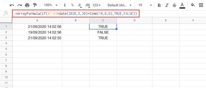
To apply the above formula to a list (for example A1:A3) that contain timestamps, we can use ArrayFormula and change the reference to A1:A3.

Example:

=ArrayFormula(
     if(
        A1:A3>date(2020,9,20)+time(10,0,0),
        TRUE,
        FALSE
     )
)
Example to Using timestamp within IF function in Google Sheets

For an entire column range A1:A, additionally use IF(LEN(A1:A), as below to limit the formula to the last non-blank row.

=ArrayFormula(
     if(
        len(A1:A),
        if(
           A1:A>date(2020,9,20)+time(10,0,0),
           TRUE,
           FALSE
        ),
     )
)

Timestamp within IFS Function in Google Sheets

The datetime use in the IFS function is slightly different. To test a single cell, for example, cell A1 we can use the below IFS formula.

=IFS(
     A1>date(2020,9,20)+time(10,0,0),
     TRUE
)

If the logical_expression (here called condition1) returns TRUE, the formula would return TRUE, else the IFS would return an #N/A (no match) error.

Syntax:

IFS(condition1, value1, [condition2, …], [value2, …])

You can ignore that error or use IFNA to return another value or blank.

=ifna(
     IFS(
        A1>date(2020,9,20)+time(10,0,0),
        TRUE
     )
)

Can I use the above IFS similar to the IF array formula?

Yes! It would be like this.

=ArrayFormula(
     if(
        len(A1:A),
        IFS(
           A1:A>date(2020,9,20)+time(10,0,0),
           TRUE
        ),
     )
)
Datetime within IF function in Google Sheets - Array formula use

Datetime + One More Criterion in IF and IFS

We have learned how to use timestamp within IF as well as IFS logical functions in Google Sheets.

Here are some additional formulas.

This time other than the date, I wish to test a second value in cell B1. The values in A1 and B1 are as follows.

AB
21/09/2020 14:02:56Accepted

I want to test this time whether datetime in cell A1 is greater than 15/09/2020 10:00:00 and the text in cell B1 is “Accepted”.

For this, with IF we should use the AND function or the equivalent asterisk operator.

Using AND with IF;

=if(
     and(A1>date(2020,9,15)+time(10,0,0),B1="Accepted"),
     TRUE,
     FALSE
)

Using Asterisk with IF;

=if(
     (A1>date(2020,9,15)+time(10,0,0))*(B1="Accepted")>0,
     TRUE,
     FALSE
)

In array formula use, you must use the asterisk one. The AND won’t allow expanding the IF formula result.

This way we can use Timestamp plus one more condition within IF function in Google Sheets.

What about IFS here?

Using AND with IFS;

=ifs(
     and(A1>date(2020,9,15)+time(10,0,0),B1="Accepted"),
     TRUE
)

Using Asterisk with IFS;

=ifs(
     (A1>date(2020,9,15)+time(10,0,0))*(B1="Accepted")>0,
     TRUE
)

That’s all. Enjoy!

Prashanth KV
Prashanth KV
Your Trusted Google Sheets and Excel Guide Prashanth KV brings a wealth of experience in Google Sheets and Excel, cultivated through years of work with multinational corporations in Mumbai and Dubai. As a recognized Google Product Expert in Docs Editors, Prashanth shares his expertise through insightful blogging since 2012. Explore his blog for practical tips and guidance on maximizing your spreadsheet skills.

How to Extract Numbers from Text in Excel with Regex

You can use the REGEXEXTRACT or REGEXREPLACE functions to easily extract numbers from text...

Using OFFSET and MATCH Together in Google Sheets: Advanced Tips

One powerful and flexible way to look up values is by combining the OFFSET...

How to Use OFFSET and XMATCH Functions Together in Excel

We often use the OFFSET and XMATCH functions together to match a value in...

How to Calculate Maximum Drawdown in Excel and Google Sheets

You can use the following dynamic array formula to calculate maximum drawdown (MDD) in...

More like this

Using OFFSET and MATCH Together in Google Sheets: Advanced Tips

One powerful and flexible way to look up values is by combining the OFFSET...

Running Count with Structured References in Google Sheets

Running a count with structured references is achievable in Google Sheets tables using the...

Running Total with Structured Table References in Google Sheets

You can use two types of formulas to create a running total with structured...

LEAVE A REPLY

Please enter your comment!
Please enter your name here

This site uses Akismet to reduce spam. Learn how your comment data is processed.