Discussing how to use SUMIF/SUMIFS while excluding duplicates in Google Sheets is important, but duplicates should not be a problem in most cases.
These functions are typically employed to calculate the sum of a column based on the occurrences of specific criteria in another column.
These occurrences can be considered duplicates, right? Therefore, there’s no issue of uniqueness or duplicates when using SUMIF/SUMIFS in the usual manner.
Before we dive into how to use SUMIF or SUMIFS while excluding duplicates in Google Sheets, it’s essential to understand this concept.
You should first understand what we mean by duplicates in the context of SUMIF/SUMIFS in Google Sheets.
Duplicates in SUMIF/SUMIFS Functions: What They Are and How to Exclude Them
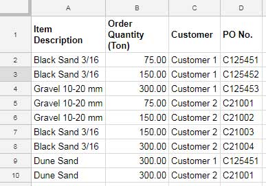
For example, consider a situation where column A contains items, column B contains ordered quantities, column C contains customer names, and column D contains purchase order numbers.

Consider the item “Black Sand 3/16,” which received four orders from two customers. Each customer ordered the item twice. However, due to a material shortage, we will only consider their first order.
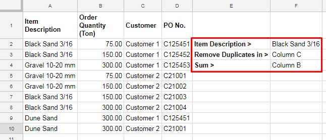
So, the purpose of SUMIF/SUMIFS here is to get the total of the item “Black Sand 3/16,” without duplicates w.r.t. customer.
Using Regular Formulas
We typically use the following formulas when we want to obtain the total orders for the item “Black Sand 3/16”:
- To get the total order of the item “Black Sand 3/16” (regardless of customer):
=SUMIF(A2:A, "Black Sand 3/16", B2:B)// returns 675=SUMIFS(B2:B, A2:A,"Black Sand 3/16")// returns 675
- If we want to get the total order of the item “Black Sand 3/16” specifically for “Customer 1”:
=SUMIFS(B2:B,A2:A,"Black Sand 3/16",C2:C,"Customer 1")// returns 225
Let’s dive into how to use SUMIF or SUMIFS while excluding duplicates in Google Sheets.
Excluding Duplicates in SUMIF/SUMIFS
Now, I’m going to discuss the topic of dealing with duplicates in SUMIF/SUMIFS calculations.
The objective is to eliminate multiple instances of the criterion based on a condition in another column.
In other words, we want to remove multiple orders of “Black Sand 3/16” from the same customer. Considering the structure of our sample data, we need to address duplicates in columns A and C.
We have two methods to achieve SUMIF/SUMIFS excluding duplicates in Google Sheets: one with a helper column and one without. We will explore both solutions.
Note: This won’t work in Excel because one of the functions used here was not available in Excel as of the last update of this post.

Using a Helper Column
I assume the above sample data is in Sheet1!A1:D.
Enter the following SORTN formula in Sheet2!A1.
=SORTN(Sheet1!A2:D,9^9,2,Sheet1!A2:A&Sheet1!C2:C,1)The SORTN function is used to eliminate duplicates. It returns unique values based on two columns, which are columns A and C.
Syntax of the SORTN Function in Google Sheets:
SORTN(range, [n], [display_ties_mode], [sort_column], [is_ascending], [sort_column2, …], [is_ascending2, …])Where:
Sheet1!A2:D: This is the range of data from which you want to remove duplicates.9^9: This number is used as an arbitrarily large number to ensure that all rows are included after processing.2: Thisdisplay_ties_modenumber indicates that you want to remove duplicates.Sheet1!A2:A&Sheet1!C2:C: This part is the key to the formula. It concatenates the values from columns A and C for each row. The repetition of these values in subsequent rows will be considered as duplicates.1: This argument specifies the sort order, with 1 indicating ascending order.
Now you can use a regular SUMIF/SUMIFS formula in this new data which contains unique records w.r.t. items and customers.
=SUMIF(A1:A,"Black Sand 3/16", B1:B)
=SUMIFS(B1:B, A1:A, "Black Sand 3/16")
This will be equivalent to excluding duplicates in the original data when using SUMIF/SUMIFS.
Formula Method Without a Helper Column
SUMIFS, as well as SUMIF, won’t work with virtual columns in the range of sum. Therefore, it’s evident that we can’t utilize the above data within these functions.
As an alternative, we can use the following QUERY:
=QUERY(SORTN(Sheet1!A2:D, 9^9, 2, Sheet1!A2:A&Sheet1!C2:C, 0), "select sum(Col2) where Col1='Black Sand 3/16' label sum(Col2)''")This QUERY calculates the sum of column 2 where the value in column 1 is equal to “Black Sand 3/16.”
So QUERY is an alternative to SUMIF/SUMIFS excluding duplicates in Google Sheets.
Conclusion
Your need to SUMIF/SUMIFS excluding duplicates may differ from the example discussed above. Nevertheless, you can consider this as a starting point.
Feel free to describe your specific requirements in the comments below. I will personally review each relevant comment.
Related: Mastering Unique Summing in Google Sheets Without SUMUNIQUEIFS.


Perfect, thank you for this!